Geometric Algebra

Some 3D renderings of the Mandelbrot set.

February 7, 2021 math and physics play , , , , ,

As mentioned previously, using geometric algebra we can convert the iterative equation for the Mandelbrot set from complex number form
\begin{equation}
z \rightarrow z^2 + c,
\end{equation}
to an equivalent vector form
\begin{equation}
\mathbf{x} \rightarrow \mathbf{x} \mathbf{e} \mathbf{x} + \mathbf{c},
\end{equation}
where \( \mathbf{e} \) represents the x-axis (say). Geometrically, each iteration takes \( \mathbf{e} \) and reflects it about the direction of \( \mathbf{x} \), then scales that by \( \mathbf{x}^2 \) and adds \( \mathbf{c} \).

To get the usual 2D Mandelbrot set, one iterates with vectors that lie only in the x-y plane, but we can treat the Mandelbrot set as a 3D solid if we remove the x-y plane restriction.

Last time I animated slices of the 3D set, but after a whole lot of messing around I managed to save the data for all the interior points of the 3D set in netCDF format, and render the solid using Paraview. Paraview has tons of filters available, and experimenting with them is pretty time consuming, but here are some initial screenshots of the 3D Mandelbrot set:

It’s interesting that much of the characteristic detail of the Mandelbrot set is not visible in the 3D volume, but if we slice that volume, you can then you can see it again.  Here’s a slice taken close to the z=0 plane (but far enough that the “CN tower” portion of the set is not visible)

You can also see some of that detail if the opacity of the rendering is turned way down:

If you look carefully at the images above, you’ll see that the axis labels are wrong.  I think that I’ve screwed up one of the stride related parameters to my putVar call, and I end up with x+z transposed in the axes labels when visualized.

Some experiments in youtube mathematics videos

January 3, 2021 math and physics play , , , , , , ,

A couple years ago I was curious how easy it would be to use a graphics tablet as a virtual chalkboard, and produced a handful of very rough YouTube videos to get a feel for the basics of streaming and video editing (much of which I’ve now forgotten how to do). These were the videos in chronological order:

  • Introduction to Geometric (Clifford) Algebra.Introduction to Geometric (Clifford) algebra. Interpretation of products of unit vectors, rules for reducing products of unit vectors, and the axioms that justify those rules.
  • Geometric Algebra: dot, wedge, cross and vector products.Geometric (Clifford) Algebra introduction, showing the relation between the vector product dot and wedge products, and the cross product.
  • Solution of two line intersection using geometric algebra.
  • Linear system solution using the wedge product.. This video provides a standalone introduction to the wedge product, the geometry of the wedge product and some properties, and linear system solution as a sample application. In this video the wedge product is introduced independently of any geometric (Clifford) algebra, as an antisymmetric and associative operator. You’ll see that we get Cramer’s rule for free from this solution technique.
  • Exponential form of vector products in geometric algebra.In this video, I discussed the exponential form of the product of two vectors.

    I showed an example of how two unit vectors, each rotations of zcap orthonormal \(\mathbb{R}^3\) planes, produce a “complex” exponential in the plane that spans these two vectors.

  • Velocity and acceleration in cylindrical coordinates using geometric algebra.I derived the cylindrical coordinate representations of the velocity and acceleration vectors, showing the radial and azimuthal components of each vector.

    I also showed how these are related to the dot and wedge product with the radial unit vector.

  • Duality transformations in geometric algebra.Duality transformations (pseudoscalar multiplication) will be demonstrated in \(\mathbb{R}^2\) and \(\mathbb{R}^3\).

    A polar parameterized vector in \(\mathbb{R}^2\), written in complex exponential form, is multiplied by a unit pseudoscalar for the x-y plane. We see that the result is a vector normal to that vector, with the direction of the normal dependent on the order of multiplication, and the orientation of the pseudoscalar used.

    In \(\mathbb{R}^3\) we see that a vector multiplied by a pseudoscalar yields the bivector that represents the plane that is normal to that vector. The sign of that bivector (or its cyclic orientation) depends on the orientation of the pseudoscalar. The order of multiplication was not mentioned in this case since the \(\mathbb{R}^3\) pseudoscalar commutes with any grade object (assumed, not proved). An example of a vector with two components in a plane, multiplied by a pseudoscalar was also given, which allowed for a visualization of the bivector that is normal to the original vector.

  • Math bait and switch: Fractional integer exponents.When I was a kid, my dad asked me to explain fractional exponents, and perhaps any non-positive integer exponents, to him. He objected to the idea of multiplying something by itself \(1/2\) times.

    I failed to answer the question to his satisfaction. My own son is now reviewing the rules of exponentiation, and it occurred to me (30 years later) why my explanation to Dad failed.

    Essentially, there’s a small bait and switch required, and my dad didn’t fall for it.

    The meaning that my dad gave to exponentiation was that \( x^n\) equals \(x\) times itself \(n\) times.

    Using this rule, it is easy to demonstrate that \(x^a x^b = x^{a + b}\), and this can be used to justify expressions like \(x^{1/2}\). However, doing this really means that we’ve switched the definition of exponential, defining an exponential as any number that satisfies the relationship:

    \(x^a x^b = x^{a+b}\),

    where \(x^1 = x\). This slight of hand is required to give meaning to \(x^{1/2}\) or other exponentials where the exponential argument is any non-positive integer.

Of these videos I just relistened to the wedge product episode, as I had a new lone comment on it, and I couldn’t even remember what I had said. It wasn’t completely horrible, despite the low tech. I was, however, very surprised how soft and gentle my voice was. When I am talking math in person, I get very animated, but attempting to manage the tech was distracting and all the excitement that I’d normally have was obliterated.

I’d love to attempt a manim based presentation of some of this material, but suspect if I do something completely scripted like that, I may not be a very good narrator.

New version of classical mechanics notes

January 1, 2021 Uncategorized , , , , , , , , ,

I’ve posted a new version of my classical mechanics notes compilation.  This version is not yet live on amazon, but you shouldn’t buy a copy of this “book” anyways, as it is horribly rough (if you want a copy, grab the free PDF instead.)  [I am going to buy a copy so that I can continue to edit a paper copy of it, but nobody else should.]

This version includes additional background material on Space Time Algebra (STA), i.e. the geometric algebra name for the Dirac/Clifford-algebra in 3+1 dimensions.  In particular, I’ve added material on reciprocal frames, the gradient and vector derivatives, line and surface integrals and the fundamental theorem for both.  Some of the integration theory content might make sense to move to a different book, but I’ll keep it with the rest of these STA notes for now.

A couple more reciprocal frame examples.

December 14, 2020 math and physics play , , , , , , , , , , , , ,

[If mathjax doesn’t display properly for you, click here for a PDF of this post]

This post logically follows both of the following:

  1. Curvilinear coordinates and gradient in spacetime, and reciprocal frames, and
  2. Lorentz transformations in Space Time Algebra (STA)

The PDF linked above above contains all the content from this post plus (1.) above [to be edited later into a more logical sequence.]

More examples.

Here are a few additional examples of reciprocal frame calculations.

Problem: Unidirectional arbitrary functional dependence.

Let
\begin{equation}\label{eqn:reciprocal:2540}
x = a f(u),
\end{equation}
where \( a \) is a constant vector and \( f(u)\) is some arbitrary differentiable function with a non-zero derivative in the region of interest.

Answer

Here we have just a single tangent space direction (a line in spacetime) with tangent vector
\begin{equation}\label{eqn:reciprocal:2400}
\Bx_u = a \PD{u}{f} = a f_u,
\end{equation}
so we see that the tangent space vectors are just rescaled values of the direction vector \( a \).
This is a simple enough parameterization that we can compute the reciprocal frame vector explicitly using the gradient. We expect that \( \Bx^u = 1/\Bx_u \), and find
\begin{equation}\label{eqn:reciprocal:2420}
\inv{a} \cdot x = f(u),
\end{equation}
but for constant \( a \), we know that \( \grad a \cdot x = a \), so taking gradients of both sides we find
\begin{equation}\label{eqn:reciprocal:2440}
\inv{a} = \grad f = \PD{u}{f} \grad u,
\end{equation}
so the reciprocal vector is
\begin{equation}\label{eqn:reciprocal:2460}
\Bx^u = \grad u = \inv{a f_u},
\end{equation}
as expected.

Problem: Linear two variable parameterization.

Let \( x = a u + b v \), where \( x \wedge a \wedge b = 0 \) represents spacetime plane (also the tangent space.) Find the curvilinear coordinates and their reciprocals.

Answer

The frame vectors are easy to compute, as they are just
\begin{equation}\label{eqn:reciprocal:1960}
\begin{aligned}
\Bx_u &= \PD{u}{x} = a \\
\Bx_v &= \PD{v}{x} = b.
\end{aligned}
\end{equation}
This is an example of a parametric equation that we can easily invert, as we have
\begin{equation}\label{eqn:reciprocal:1980}
\begin{aligned}
x \wedge a &= – v \lr{ a \wedge b } \\
x \wedge b &= u \lr{ a \wedge b },
\end{aligned}
\end{equation}
so
\begin{equation}\label{eqn:reciprocal:2000}
\begin{aligned}
u
&= \inv{ a \wedge b } \cdot \lr{ x \wedge b } \\
&= \inv{ \lr{a \wedge b}^2 } \lr{ a \wedge b } \cdot \lr{ x \wedge b } \\
&=
\frac{
\lr{b \cdot x} \lr{ a \cdot b }

\lr{a \cdot x} \lr{ b \cdot b }
}{ \lr{a \wedge b}^2 }
\end{aligned}
\end{equation}
\begin{equation}\label{eqn:reciprocal:2020}
\begin{aligned}
v &= -\inv{ a \wedge b } \cdot \lr{ x \wedge a } \\
&= -\inv{ \lr{a \wedge b}^2 } \lr{ a \wedge b } \cdot \lr{ x \wedge a } \\
&=
-\frac{
\lr{b \cdot x} \lr{ a \cdot a }

\lr{a \cdot x} \lr{ a \cdot b }
}{ \lr{a \wedge b}^2 }
\end{aligned}
\end{equation}
Recall that \( \grad \lr{ a \cdot x} = a \), if \( a \) is a constant, so our gradients are just
\begin{equation}\label{eqn:reciprocal:2040}
\begin{aligned}
\grad u
&=
\frac{
b \lr{ a \cdot b }

a
\lr{ b \cdot b }
}{ \lr{a \wedge b}^2 } \\
&=
b \cdot \inv{ a \wedge b },
\end{aligned}
\end{equation}
and
\begin{equation}\label{eqn:reciprocal:2060}
\begin{aligned}
\grad v
&=
-\frac{
b \lr{ a \cdot a }

a \lr{ a \cdot b }
}{ \lr{a \wedge b}^2 } \\
&=
-a \cdot \inv{ a \wedge b }.
\end{aligned}
\end{equation}
Expressed in terms of the frame vectors, this is just
\begin{equation}\label{eqn:reciprocal:2080}
\begin{aligned}
\Bx^u &= \Bx_v \cdot \inv{ \Bx_u \wedge \Bx_v } \\
\Bx^v &= -\Bx_u \cdot \inv{ \Bx_u \wedge \Bx_v },
\end{aligned}
\end{equation}
so we were able to show, for this special two parameter linear case, that the explicit evaluation of the gradients has the exact structure that we intuited that the reciprocals must have, provided they are constrained to the spacetime plane \( a \wedge b \). It is interesting to observe how this structure falls out of the linear system solution so directly. Also note that these reciprocals are not defined at the origin of the \( (u,v) \) parameter space.

Problem: Quadratic two variable parameterization.

Now consider a variation of the previous problem, with \( x = a u^2 + b v^2 \). Find the curvilinear coordinates and their reciprocals.

Answer

\begin{equation}\label{eqn:reciprocal:2100}
\begin{aligned}
\Bx_u &= \PD{u}{x} = 2 u a \\
\Bx_v &= \PD{v}{x} = 2 v b.
\end{aligned}
\end{equation}
Our tangent space is still the \( a \wedge b \) plane (as is the surface itself), but the spacing of the cells starts getting wider in proportion to \( u, v \).
Utilizing the work from the previous problem, we have
\begin{equation}\label{eqn:reciprocal:2120}
\begin{aligned}
2 u \grad u &=
b \cdot \inv{ a \wedge b } \\
2 v \grad v &=
-a \cdot \inv{ a \wedge b }.
\end{aligned}
\end{equation}
A bit of rearrangement can show that this is equivalent to the reciprocal frame identities. This is a second demonstration that the gradient and the algebraic formulations for the reciprocals match, at least for these special cases of linear non-coupled parameterizations.

Problem: Reciprocal frame for generalized cylindrical parameterization.

Let the vector parameterization be \( x(\rho,\theta) = \rho e^{-i\theta/2} x(\rho_0, \theta_0) e^{i \theta} \), where \( i^2 = \pm 1 \) is a unit bivector (\(+1\) for a boost, and \(-1\) for a rotation), and where \(\theta, \rho\) are scalars. Find the tangent space vectors and their reciprocals.

fig. 1. “Cylindrical” boost parameterization.

Note that this is cylindrical parameterization for the rotation case, and traces out hyperbolic regions for the boost case. The boost case is illustrated in fig. 1 where hyperbolas in the light cone are found for boosts of \( \gamma_0\) with various values of \(\rho\), and the spacelike hyperbolas are boosts of \( \gamma_1 \), again for various values of \( \rho \).

Answer

The tangent space vectors are
\begin{equation}\label{eqn:reciprocal:2480}
\Bx_\rho = \frac{x}{\rho},
\end{equation}
and

\begin{equation}\label{eqn:reciprocal:2500}
\begin{aligned}
\Bx_\theta
&= -\frac{i}{2} x + x \frac{i}{2} \\
&= x \cdot i.
\end{aligned}
\end{equation}
Recall that \( x \cdot i \) lies perpendicular to \( x \) (in the plane \( i \)), as illustrated in fig. 2. This means that \( \Bx_\rho \) and \( \Bx_\theta \) are orthogonal, so we can find the reciprocal vectors by just inverting them
\begin{equation}\label{eqn:reciprocal:2520}
\begin{aligned}
\Bx^\rho &= \frac{\rho}{x} \\
\Bx^\theta &= \frac{1}{x \cdot i}.
\end{aligned}
\end{equation}

fig. 2. Projection and rejection geometry.

Parameterization of a general linear transformation.

Given \( N \) parameters \( u^0, u^1, \cdots u^{N-1} \), a general linear transformation from the parameter space to the vector space has the form
\begin{equation}\label{eqn:reciprocal:2160}
x =
{a^\alpha}_\beta \gamma_\alpha u^\beta,
\end{equation}
where \( \beta \in [0, \cdots, N-1] \) and \( \alpha \in [0,3] \).
For such a general transformation, observe that the curvilinear basis vectors are
\begin{equation}\label{eqn:reciprocal:2180}
\begin{aligned}
\Bx_\mu
&= \PD{u^\mu}{x} \\
&= \PD{u^\mu}{}
{a^\alpha}_\beta \gamma_\alpha u^\beta \\
&=
{a^\alpha}_\mu \gamma_\alpha.
\end{aligned}
\end{equation}
We find an interpretation of \( {a^\alpha}_\mu \) by dotting \( \Bx_\mu \) with the reciprocal frame vectors of the standard basis
\begin{equation}\label{eqn:reciprocal:2200}
\begin{aligned}
\Bx_\mu \cdot \gamma^\nu
&=
{a^\alpha}_\mu \lr{ \gamma_\alpha \cdot \gamma^\nu } \\
&=
{a^\nu}_\mu,
\end{aligned}
\end{equation}
so
\begin{equation}\label{eqn:reciprocal:2220}
x = \Bx_\mu u^\mu.
\end{equation}
We are able to reinterpret \ref{eqn:reciprocal:2160} as a contraction of the tangent space vectors with the parameters, scaling and summing these direction vectors to characterize all the points in the tangent plane.

Theorem 1.1: Projecting onto the tangent space.

Let \( T \) represent the tangent space. The projection of a vector onto the tangent space has the form
\begin{equation}\label{eqn:reciprocal:2560}
\textrm{Proj}_{\textrm{T}} y = \lr{ y \cdot \Bx^\mu } \Bx_\mu = \lr{ y \cdot \Bx_\mu } \Bx^\mu.
\end{equation}

Start proof:

Let’s designate \( a \) as the portion of the vector \( y \) that lies outside of the tangent space
\begin{equation}\label{eqn:reciprocal:2260}
y = y^\mu \Bx_\mu + a.
\end{equation}
If we knew the coordinates \( y^\mu \), we would have a recipe for the projection.
Algebraically, requiring that \( a \) lies outside of the tangent space, is equivalent to stating \( a \cdot \Bx_\mu = a \cdot \Bx^\mu = 0 \). We use that fact, and then take dot products
\begin{equation}\label{eqn:reciprocal:2280}
\begin{aligned}
y \cdot \Bx^\nu
&= \lr{ y^\mu \Bx_\mu + a } \cdot \Bx^\nu \\
&= y^\nu,
\end{aligned}
\end{equation}
so
\begin{equation}\label{eqn:reciprocal:2300}
y = \lr{ y \cdot \Bx^\mu } \Bx_\mu + a.
\end{equation}
Similarly, the tangent space projection can be expressed as a linear combination of reciprocal basis elements
\begin{equation}\label{eqn:reciprocal:2320}
y = y_\mu \Bx^\mu + a.
\end{equation}
Dotting with \( \Bx_\mu \), we have
\begin{equation}\label{eqn:reciprocal:2340}
\begin{aligned}
y \cdot \Bx^\mu
&= \lr{ y_\alpha \Bx^\alpha + a } \cdot \Bx_\mu \\
&= y_\mu,
\end{aligned}
\end{equation}
so
\begin{equation}\label{eqn:reciprocal:2360}
y = \lr{ y \cdot \Bx^\mu } \Bx_\mu + a.
\end{equation}
We find the two stated ways of computing the projection.

Observe that, for the special case that all of \( \setlr{ \Bx_\mu } \) are orthogonal, the equivalence of these two projection methods follows directly, since
\begin{equation}\label{eqn:reciprocal:2380}
\begin{aligned}
\lr{ y \cdot \Bx^\mu } \Bx_\mu
&=
\lr{ y \cdot \inv{\Bx_\mu} } \inv{\Bx^\mu} \\
&=
\lr{ y \cdot \frac{\Bx_\mu}{\lr{\Bx_\mu}^2 } } \frac{\Bx^\mu}{\lr{\Bx^\mu}^2} \\
&=
\lr{ y \cdot \Bx_\mu } \Bx^\mu.
\end{aligned}
\end{equation}

End proof.

Lorentz transformations in Space Time Algebra (STA)

December 12, 2020 math and physics play , , , , , , , , , , , , , , , , , ,

[If mathjax doesn’t display properly for you, click here for a PDF of this post]

Motivation.

One of the remarkable features of geometric algebra are the complex exponential sandwiches that can be used to encode rotations in any dimension, or rotation like operations like Lorentz transformations in Minkowski spaces. In this post, we show some examples that unpack the geometric algebra expressions for Lorentz transformations operations of this sort. In particular, we will look at the exponential sandwich operations for spatial rotations and Lorentz boosts in the Dirac algebra, known as Space Time Algebra (STA) in geometric algebra circles, and demonstrate that these sandwiches do have the desired effects.

Lorentz transformations.

Theorem 1.1: Lorentz transformation.

The transformation
\begin{equation}\label{eqn:lorentzTransform:580}
x \rightarrow e^{B} x e^{-B} = x’,
\end{equation}
where \( B = a \wedge b \), is an STA 2-blade for any two linearly independent four-vectors \( a, b \), is a norm preserving, that is
\begin{equation}\label{eqn:lorentzTransform:600}
x^2 = {x’}^2.
\end{equation}

Start proof:

The proof is disturbingly trivial in this geometric algebra form
\begin{equation}\label{eqn:lorentzTransform:40}
\begin{aligned}
{x’}^2
&=
e^{B} x e^{-B} e^{B} x e^{-B} \\
&=
e^{B} x x e^{-B} \\
&=
x^2 e^{B} e^{-B} \\
&=
x^2.
\end{aligned}
\end{equation}

End proof.

In particular, observe that we did not need to construct the usual infinitesimal representations of rotation and boost transformation matrices or tensors in order to demonstrate that we have spacetime invariance for the transformations. The rough idea of such a transformation is that the exponential commutes with components of the four-vector that lie off the spacetime plane specified by the bivector \( B \), and anticommutes with components of the four-vector that lie in the plane. The end result is that the sandwich operation simplifies to
\begin{equation}\label{eqn:lorentzTransform:60}
x’ = x_\parallel e^{-B} + x_\perp,
\end{equation}
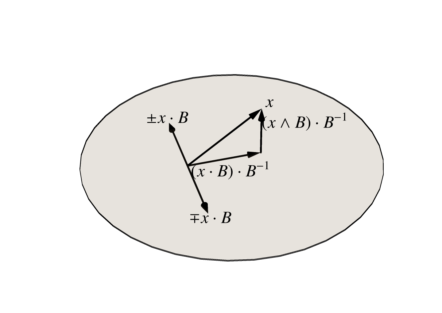
where \( x = x_\perp + x_\parallel \) and \( x_\perp \cdot B = 0 \), and \( x_\parallel \wedge B = 0 \). In particular, using \( x = x B B^{-1} = \lr{ x \cdot B + x \wedge B } B^{-1} \), we find that
\begin{equation}\label{eqn:lorentzTransform:80}
\begin{aligned}
x_\parallel &= \lr{ x \cdot B } B^{-1} \\
x_\perp &= \lr{ x \wedge B } B^{-1}.
\end{aligned}
\end{equation}
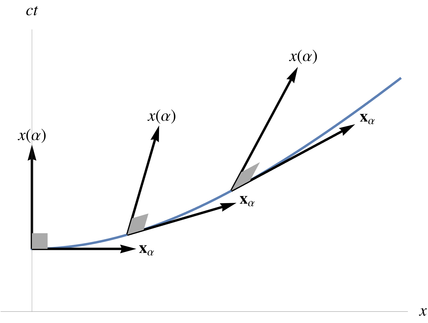
When \( B \) is a spacetime plane \( B = b \wedge \gamma_0 \), then this exponential has a hyperbolic nature, and we end up with a Lorentz boost. When \( B \) is a spatial bivector, we end up with a single complex exponential, encoding our plane old 3D rotation. More general \( B \)’s that encode composite boosts and rotations are also possible, but \( B \) must be invertible (it should have no lightlike factors.) The rough geometry of these projections is illustrated in fig 1, where the spacetime plane is represented by \( B \).

Projection and rejection geometry.

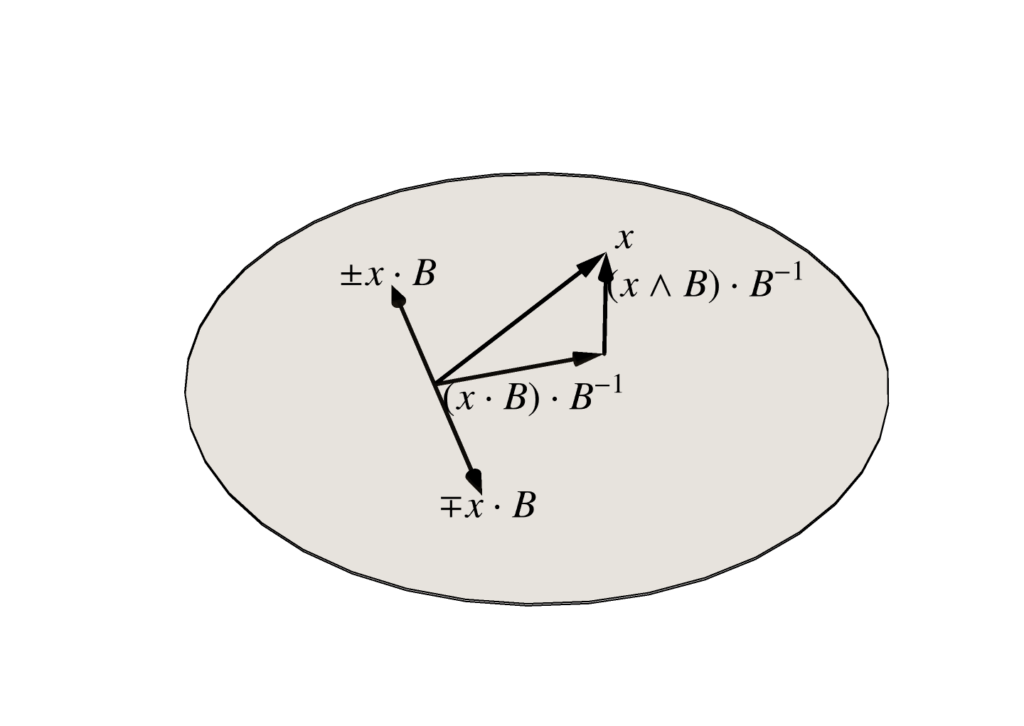
fig 1. Projection and rejection geometry.


What is not so obvious is how to pick \( B \)’s that correspond to specific rotation axes or boost directions. Let’s consider each of those cases in turn.

Theorem 1.2: Boost.

The boost along a direction vector \( \vcap \) and rapidity \( \alpha \) is given by
\begin{equation}\label{eqn:lorentzTransform:620}
x’ = e^{-\vcap \alpha/2} x e^{\vcap \alpha/2},
\end{equation}
where \( \vcap = \gamma_{k0} \cos\theta^k \) is an STA bivector representing a spatial direction with direction cosines \( \cos\theta^k \).

Start proof:

We want to demonstrate that this is equivalent to the usual boost formulation. We can start with decomposition of the four-vector \( x \) into components that lie in and off of the spacetime plane \( \vcap \).
\begin{equation}\label{eqn:lorentzTransform:100}
\begin{aligned}
x
&= \lr{ x^0 + \Bx } \gamma_0 \\
&= \lr{ x^0 + \Bx \vcap^2 } \gamma_0 \\
&= \lr{ x^0 + \lr{ \Bx \cdot \vcap} \vcap + \lr{ \Bx \wedge \vcap} \vcap } \gamma_0,
\end{aligned}
\end{equation}
where \( \Bx = x \wedge \gamma_0 \). The first two components lie in the boost plane, whereas the last is the spatial component of the vector that lies perpendicular to the boost plane. Observe that \( \vcap \) anticommutes with the dot product term and commutes with he wedge product term, so we have
\begin{equation}\label{eqn:lorentzTransform:120}
\begin{aligned}
x’
&=
\lr{ x^0 + \lr{ \Bx \cdot \vcap } \vcap } \gamma_0
e^{\vcap \alpha/2 }
e^{\vcap \alpha/2 }
+
\lr{ \Bx \wedge \vcap } \vcap \gamma_0
e^{-\vcap \alpha/2 }
e^{\vcap \alpha/2 } \\
&=
\lr{ x^0 + \lr{ \Bx \cdot \vcap } \vcap } \gamma_0
e^{\vcap \alpha }
+
\lr{ \Bx \wedge \vcap } \vcap \gamma_0.
\end{aligned}
\end{equation}
Noting that \( \vcap^2 = 1 \), we may expand the exponential in hyperbolic functions, and find that the boosted portion of the vector expands as
\begin{equation}\label{eqn:lorentzTransform:260}
\begin{aligned}
\lr{ x^0 + \lr{ \Bx \cdot \vcap} \vcap } \gamma_0 e^{\vcap \alpha}
&=
\lr{ x^0 + \lr{ \Bx \cdot \vcap} \vcap } \gamma_0 \lr{ \cosh\alpha + \vcap \sinh \alpha} \\
&=
\lr{ x^0 + \lr{ \Bx \cdot \vcap} \vcap } \lr{ \cosh\alpha – \vcap \sinh \alpha} \gamma_0 \\
&=
\lr{ x^0 \cosh\alpha – \lr{ \Bx \cdot \vcap} \sinh \alpha} \gamma_0
+
\lr{ -x^0 \sinh \alpha + \lr{ \Bx \cdot \vcap} \cosh \alpha } \vcap \gamma_0.
\end{aligned}
\end{equation}
We are left with
\begin{equation}\label{eqn:lorentzTransform:320}
\begin{aligned}
x’
&=
\lr{ x^0 \cosh\alpha – \lr{ \Bx \cdot \vcap} \sinh \alpha} \gamma_0
+
\lr{ \lr{ \Bx \cdot \vcap} \cosh \alpha -x^0 \sinh \alpha } \vcap \gamma_0
+
\lr{ \Bx \wedge \vcap} \vcap \gamma_0 \\
&=
\begin{bmatrix}
\gamma_0 & \vcap \gamma_0
\end{bmatrix}
\begin{bmatrix}
\cosh\alpha & – \sinh\alpha \\
-\sinh\alpha & \cosh\alpha
\end{bmatrix}
\begin{bmatrix}
x^0 \\
\Bx \cdot \vcap
\end{bmatrix}
+
\lr{ \Bx \wedge \vcap} \vcap \gamma_0,
\end{aligned}
\end{equation}
which has the desired Lorentz boost structure. Of course, this is usually seen with \( \vcap = \gamma_{10} \) so that the components in the coordinate column vector are \( (ct, x) \).

End proof.

Theorem 1.3: Spatial rotation.

Given two linearly independent spatial bivectors \( \Ba = a^k \gamma_{k0}, \Bb = b^k \gamma_{k0} \), a rotation of \(\theta\) radians in the plane of \( \Ba, \Bb \) from \( \Ba \) towards \( \Bb \), is given by
\begin{equation}\label{eqn:lorentzTransform:640}
x’ = e^{-i\theta} x e^{i\theta},
\end{equation}
where \( i = (\Ba \wedge \Bb)/\Abs{\Ba \wedge \Bb} \), is a unit (spatial) bivector.

Start proof:

Without loss of generality, we may pick \( i = \acap \bcap \), where \( \acap^2 = \bcap^2 = 1 \), and \( \acap \cdot \bcap = 0 \). With such an orthonormal basis for the plane, we can decompose our four vector into portions that lie in and off the plane
\begin{equation}\label{eqn:lorentzTransform:400}
\begin{aligned}
x
&= \lr{ x^0 + \Bx } \gamma_0 \\
&= \lr{ x^0 + \Bx i i^{-1} } \gamma_0 \\
&= \lr{ x^0 + \lr{ \Bx \cdot i } i^{-1} + \lr{ \Bx \wedge i } i^{-1} } \gamma_0.
\end{aligned}
\end{equation}
The projective term lies in the plane of rotation, whereas the timelike and spatial rejection term are perpendicular. That is
\begin{equation}\label{eqn:lorentzTransform:420}
\begin{aligned}
x_\parallel &= \lr{ \Bx \cdot i } i^{-1} \gamma_0 \\
x_\perp &= \lr{ x^0 + \lr{ \Bx \wedge i } i^{-1} } \gamma_0,
\end{aligned}
\end{equation}
where \( x_\parallel \wedge i = 0 \), and \( x_\perp \cdot i = 0 \). The plane pseudoscalar \( i \) anticommutes with \( x_\parallel \), and commutes with \( x_\perp \), so
\begin{equation}\label{eqn:lorentzTransform:440}
\begin{aligned}
x’
&= e^{-i\theta/2} \lr{ x_\parallel + x_\perp } e^{i\theta/2} \\
&= x_\parallel e^{i\theta} + x_\perp.
\end{aligned}
\end{equation}
However
\begin{equation}\label{eqn:lorentzTransform:460}
\begin{aligned}
\lr{ \Bx \cdot i } i^{-1}
&=
\lr{ \Bx \cdot \lr{ \acap \wedge \bcap } } \bcap \acap \\
&=
\lr{\Bx \cdot \acap} \bcap \bcap \acap
-\lr{\Bx \cdot \bcap} \acap \bcap \acap \\
&=
\lr{\Bx \cdot \acap} \acap
+\lr{\Bx \cdot \bcap} \bcap,
\end{aligned}
\end{equation}
so
\begin{equation}\label{eqn:lorentzTransform:480}
\begin{aligned}
x_\parallel e^{i\theta}
&=
\lr{
\lr{\Bx \cdot \acap} \acap
+
\lr{\Bx \cdot \bcap} \bcap
}
\gamma_0
\lr{
\cos\theta + \acap \bcap \sin\theta
} \\
&=
\acap \lr{
\lr{\Bx \cdot \acap} \cos\theta

\lr{\Bx \cdot \bcap} \sin\theta
}
\gamma_0
+
\bcap \lr{
\lr{\Bx \cdot \acap} \sin\theta
+
\lr{\Bx \cdot \bcap} \cos\theta
}
\gamma_0,
\end{aligned}
\end{equation}
so
\begin{equation}\label{eqn:lorentzTransform:500}
x’
=
\begin{bmatrix}
\acap & \bcap
\end{bmatrix}
\begin{bmatrix}
\cos\theta & – \sin\theta \\
\sin\theta & \cos\theta
\end{bmatrix}
\begin{bmatrix}
\Bx \cdot \acap \\
\Bx \cdot \bcap \\
\end{bmatrix}
\gamma_0
+
\lr{ x \wedge i} i^{-1} \gamma_0.
\end{equation}
Observe that this rejection term can be explicitly expanded to
\begin{equation}\label{eqn:lorentzTransform:520}
\lr{ \Bx \wedge i} i^{-1} \gamma_0 =
x –
\lr{ \Bx \cdot \acap } \acap \gamma_0

\lr{ \Bx \cdot \acap } \acap \gamma_0.
\end{equation}
This is the timelike component of the vector, plus the spatial component that is normal to the plane. This exponential sandwich transformation rotates only the portion of the vector that lies in the plane, and leaves the rest (timelike and normal) untouched.

End proof.

Problems.

Problem: Verify components relative to boost direction.

In the proof of thm. 1.2, the vector \( x \) was expanded in terms of the spacetime split. An alternate approach, is to expand as
\begin{equation}\label{eqn:lorentzTransform:340}
\begin{aligned}
x
&= x \vcap^2 \\
&= \lr{ x \cdot \vcap + x \wedge \vcap } \vcap \\
&= \lr{ x \cdot \vcap } \vcap + \lr{ x \wedge \vcap } \vcap.
\end{aligned}
\end{equation}
Show that
\begin{equation}\label{eqn:lorentzTransform:360}
\lr{ x \cdot \vcap } \vcap
=
\lr{ x^0 + \lr{ \Bx \cdot \vcap} \vcap } \gamma_0,
\end{equation}
and
\begin{equation}\label{eqn:lorentzTransform:380}
\lr{ x \wedge \vcap } \vcap
=
\lr{ \Bx \wedge \vcap} \vcap \gamma_0.
\end{equation}

Answer

Let \( x = x^\mu \gamma_\mu \), so that
\begin{equation}\label{eqn:lorentzTransform:160}
\begin{aligned}
x \cdot \vcap
&=
\gpgradeone{ x^\mu \gamma_\mu \cos\theta^b \gamma_{b 0} } \\
&=
x^\mu \cos\theta^b \gpgradeone{ \gamma_\mu \gamma_{b 0} }
.
\end{aligned}
\end{equation}
The \( \mu = 0 \) component of this grade selection is
\begin{equation}\label{eqn:lorentzTransform:180}
\gpgradeone{ \gamma_0 \gamma_{b 0} }
=
-\gamma_b,
\end{equation}
and for \( \mu = a \ne 0 \), we have
\begin{equation}\label{eqn:lorentzTransform:200}
\gpgradeone{ \gamma_a \gamma_{b 0} }
=
-\delta_{a b} \gamma_0,
\end{equation}
so we have
\begin{equation}\label{eqn:lorentzTransform:220}
\begin{aligned}
x \cdot \vcap
&=
x^0 \cos\theta^b (-\gamma_b)
+
x^a \cos\theta^b (-\delta_{ab} \gamma_0 ) \\
&=
-x^0 \vcap \gamma_0

x^b \cos\theta^b \gamma_0 \\
&=
– \lr{ x^0 \vcap + \Bx \cdot \vcap } \gamma_0,
\end{aligned}
\end{equation}
where \( \Bx = x \wedge \gamma_0 \) is the spatial portion of the four vector \( x \) relative to the stationary observer frame. Since \( \vcap \) anticommutes with \( \gamma_0 \), the component of \( x \) in the spacetime plane \( \vcap \) is
\begin{equation}\label{eqn:lorentzTransform:240}
\lr{ x \cdot \vcap } \vcap =
\lr{ x^0 + \lr{ \Bx \cdot \vcap} \vcap } \gamma_0,
\end{equation}
as expected.

For the rejection term, we have
\begin{equation}\label{eqn:lorentzTransform:280}
x \wedge \vcap
=
x^\mu \cos\theta^s \gpgradethree{ \gamma_\mu \gamma_{s 0} }.
\end{equation}
The \( \mu = 0 \) term clearly contributes nothing, leaving us with:
\begin{equation}\label{eqn:lorentzTransform:300}
\begin{aligned}
\lr{ x \wedge \vcap } \vcap
&=
\lr{ x \wedge \vcap } \cdot \vcap \\
&=
x^r \cos\theta^s \cos\theta^t \lr{ \lr{ \gamma_r \wedge \gamma_{s}} \gamma_0 } \cdot \lr{ \gamma_{t0} } \\
&=
x^r \cos\theta^s \cos\theta^t \gpgradeone{
\lr{ \gamma_r \wedge \gamma_{s} } \gamma_0 \gamma_{t0}
} \\
&=
-x^r \cos\theta^s \cos\theta^t \lr{ \gamma_r \wedge \gamma_{s}} \cdot \gamma_t \\
&=
-x^r \cos\theta^s \cos\theta^t \lr{ -\gamma_r \delta_{st} + \gamma_s \delta_{rt} } \\
&=
x^r \cos\theta^t \cos\theta^t \gamma_r

x^t \cos\theta^s \cos\theta^t \gamma_s \\
&=
\Bx \gamma_0
– (\Bx \cdot \vcap) \vcap \gamma_0 \\
&=
\lr{ \Bx \wedge \vcap} \vcap \gamma_0,
\end{aligned}
\end{equation}
as expected. Is there a clever way to demonstrate this without resorting to coordinates?

Problem: Rotation transformation components.

Given a unit spatial bivector \( i = \acap \bcap \), where \( \acap \cdot \bcap = 0 \) and \( i^2 = -1 \), show that
\begin{equation}\label{eqn:lorentzTransform:540}
\lr{ x \cdot i } i^{-1}
=
\lr{ \Bx \cdot i } i^{-1} \gamma_0
=
\lr{\Bx \cdot \acap } \acap \gamma_0
+
\lr{\Bx \cdot \bcap } \bcap \gamma_0,
\end{equation}
and
\begin{equation}\label{eqn:lorentzTransform:560}
\lr{ x \wedge i } i^{-1}
=
\lr{ \Bx \wedge i } i^{-1} \gamma_0
=
x –
\lr{\Bx \cdot \acap } \acap \gamma_0

\lr{\Bx \cdot \bcap } \bcap \gamma_0.
\end{equation}
Also show that \( i \) anticommutes with \( \lr{ x \cdot i } i^{-1} \) and commutes with \( \lr{ x \wedge i } i^{-1} \).

Answer

This problem is left for the reader, as I don’t feel like typing out my solution.

The first part of this problem can be done in the tedious coordinate approach used above, but hopefully there is a better way.

For the last (commutation) part of the problem, here is a hint. Let \( x \wedge i = n i \), where \( n \cdot i = 0 \). The result then follows easily.