Some slices.
As followup to:
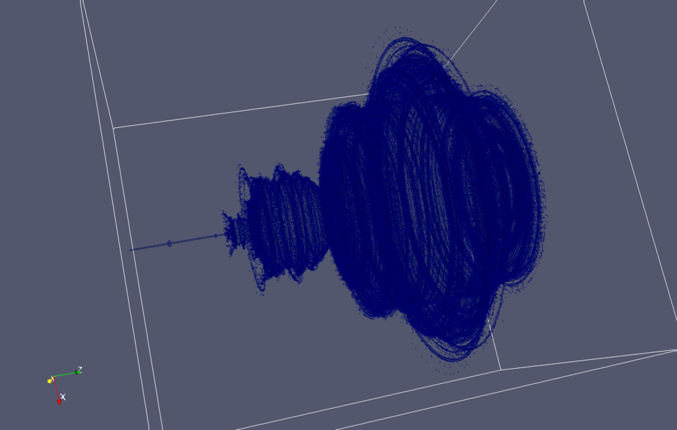
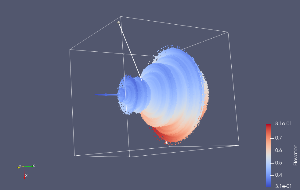
here is a bit more experimentation with Paraview slice filtering. This time I saved all the point data with the escape time counts, and rendered it with a few different contours
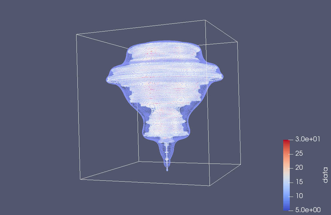
The default slice filter places the plane in the x-y orientation:
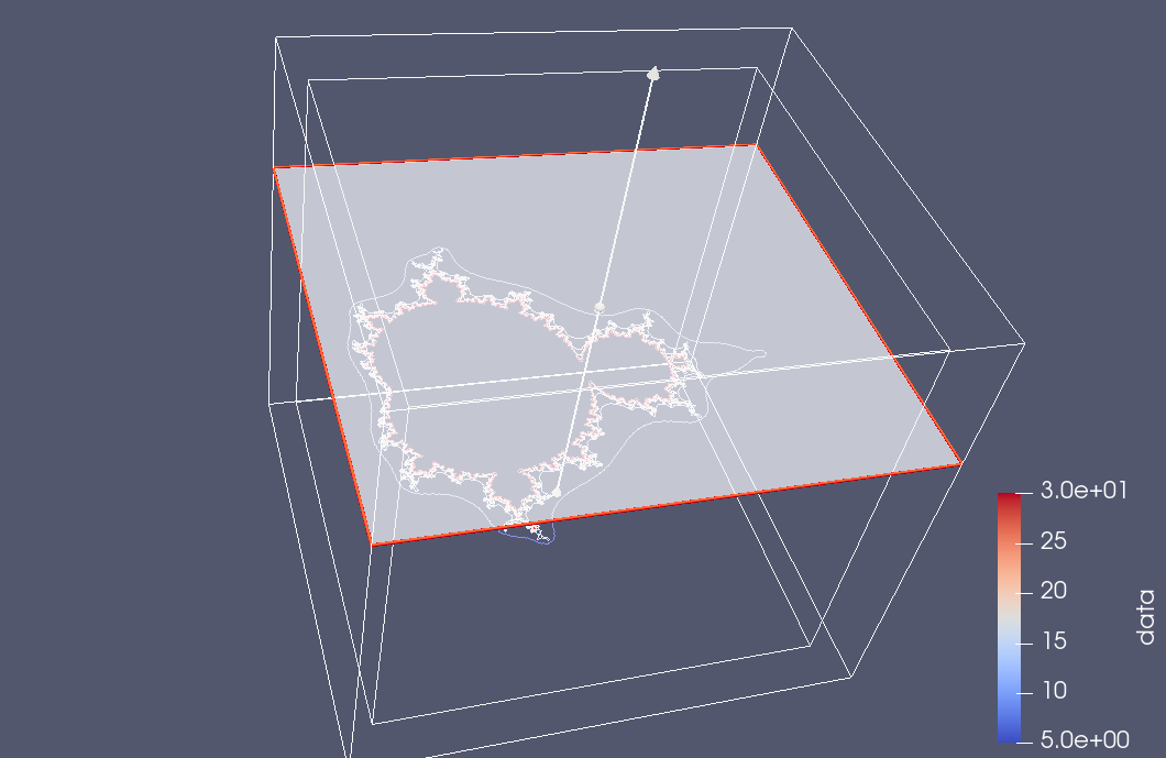
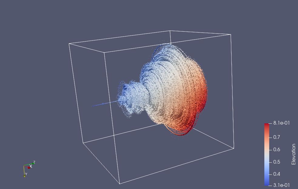
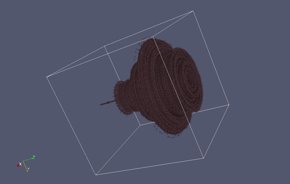
but we can also tilt it in the Paraview render UI
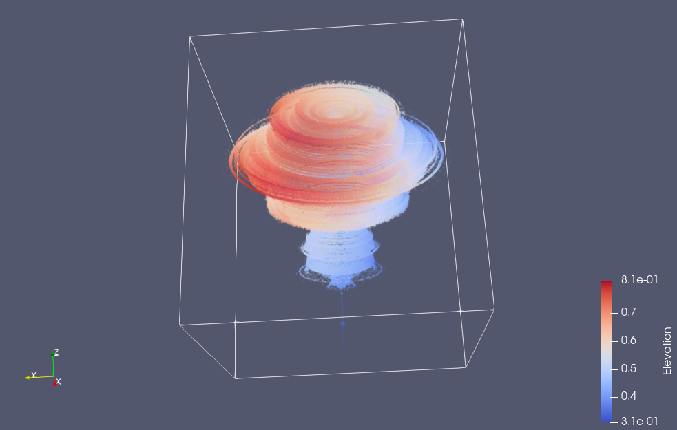
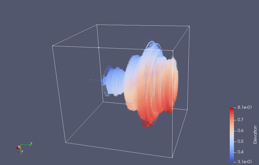
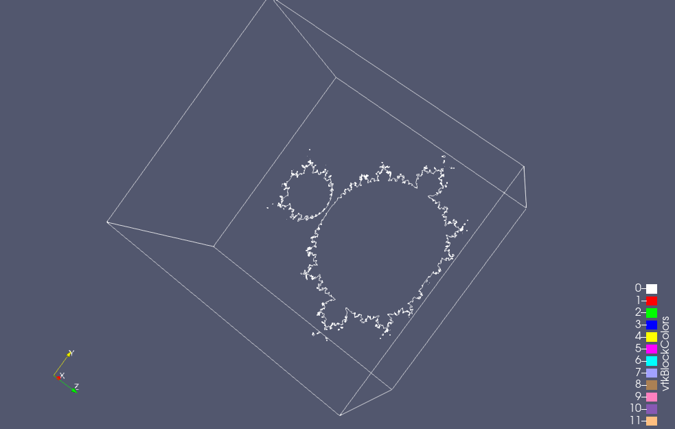
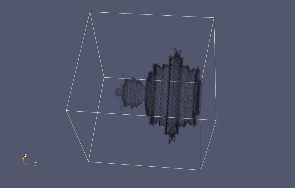
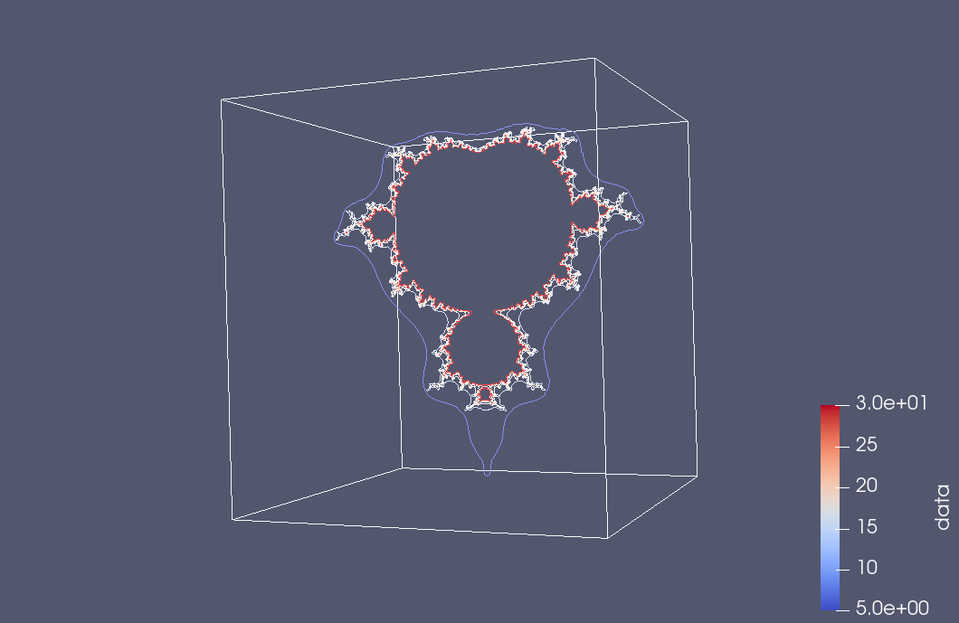
and suppress the contour view to see just the slice
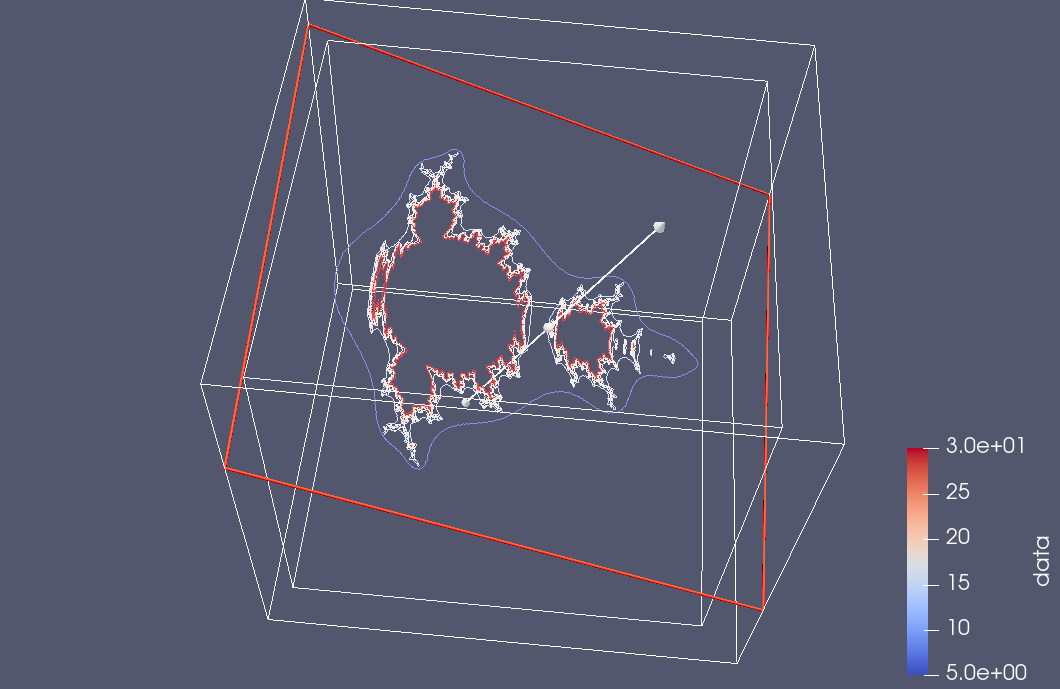
As a very GUI challenged user, I don’t find the interface particularly intuitive, but have at least figured out this one particular slicing task, which is kind of cool. It’s impressive that the UI can drive interesting computational tasks without having to regenerate or reload any of the raw data itself. This time I was using the MacOSX Paraview client, which is nicer looking than the Windows version, but has some weird glitches in the file dialogues.
Analysis.
The graphing play above shows some apparent rotational symmetry our vector equivalent to the Mandelbrot equation
\begin{equation}
\Bx \rightarrow \Bx \Be_1 \Bx + \Bc.
\end{equation}
It was not clear to me if this symmetry existed, as there were artifacts in the plots that made it appear that there was irregularity. However, some thought shows that this irregularity is strictly due to sampling error, and perhaps also due to limitations in the plotting software, as such an uneven surface is probably tricky to deal with.
To see this, here are the first few iterations of the Mandlebrot sequence for an arbitary starting vector \( \Bc \).
\begin{equation}
\begin{aligned}
\Bx_0 &= \Bc \\
\Bx_1 &= \Bc \Be_1 \Bc + \Bc \\
\Bx_2 &= \lr{ \Bc \Be_1 \Bc + \Bc } \Be_1 \lr{ \Bc \Be_1 \Bc + \Bc } + \Bc \Be_1 \Bc + \Bc.
\end{aligned}
\end{equation}
Now, what happens when we rotate the starting vector \( \Bc \) in the \( y-z \) plane. The rotor for such a rotation is
\begin{equation}
R = \exp\lr{ e_{23} \theta/2 },
\end{equation}
where
\begin{equation}
\Bc \rightarrow R \Bc \tilde{R}.
\end{equation}
Observe that if \( \Bc \) is parallel to the x-axis, then this rotation leaves the starting point invariant, as \( \Be_1 \) commutes with \( R \). That is
\begin{equation}
R \Be_1 \tilde{R} =
\Be_1 R \tilde{R} = \Be_1.
\end{equation}
Let \( \Bc’ = R \Bc \tilde{R} \), so that
\begin{equation}
\Bx_0′ = R \Bc \tilde{R} = R \Bx_0 \tilde{R} .
\end{equation}
\begin{equation}
\begin{aligned}
\Bx_1′
&= R \Bc \tilde{R} \Be_1 R \Bc \tilde{R} + R \Bc \tilde{R} \\
&= R \Bc \Be_1 \Bc \tilde{R} + R \Bc \tilde{R} \\
&= R \lr{ \Bc \Be_1 \Bc R + \Bc } \tilde{R} \\
&= R \Bx_1 \tilde{R}.
\end{aligned}
\end{equation}
\begin{equation}\label{eqn:m2:n}
\begin{aligned}
\Bx_2′
&= \Bx_1′ \Be_1 \Bx_1′ + \Bc’ \\
&= R \Bx_1 \tilde{R} \Be_1 R \Bx_1 \tilde{R} + R \Bc \tilde{R} \\
&= R \Bx_1 \Be_1 \Bx_1 \tilde{R} + R \Bc \tilde{R} \\
&= R \lr{ \Bx_1 \Be_1 \Bx_1 + \Bc } \tilde{R} \\
&= R \Bx_2 \tilde{R}.
\end{aligned}
\end{equation}
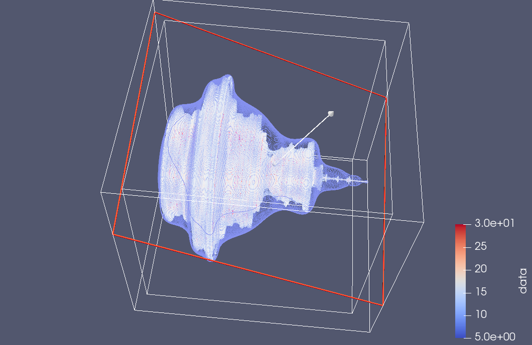
The pattern is clear. If we rotate the starting point in the y-z plane, iterating the Mandelbrot sequence results in precisely the same rotation of the x-y plane Mandelbrot sequence. So the apparent rotational symmetry in the 3D iteration of the Mandelbrot vector equation is exactly that. This is an unfortunately boring 3D fractal. All of the interesting fractal nature occurs in the 2D plane, and the rest is just a consequence of rotating that image around the x-axis. We get some interesting fractal artifacts if we slice the rotated Mandelbrot image.