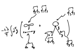
scattering

My old Quantum II notes are now available on amazon

May 17, 2020 phy456 , , , , , , , , ,

PHY456, Quantum Mechanics II was one of the first few courses that I did as part of my non-degree upper year physics program.  That was a self directed study part time program, where I took most of interesting seeming fourth year undergrad physics courses at UofT.

I was never really pleased with how my QMII notes came out, and unlike some of my other notes compilations, I never made a version available on amazon, instead just had the PDF available for free on my Quantum Mechanics page.  That page also outlines how to get a copy of the latex sources for the notes (for the curious, or for the zealous reader who wants to submit merge requests with corrections.)

Well, over the last month or so, I’ve gradually cleaned up these QMII notes enough that they are “print-ready” (no equations overflowing into the “gutter”, …) , and have gone ahead and made it available on amazon, for $10 USD.  Like my other class notes “books”, this is published using amazon’s print on demand service.  In the likely event that nobody will order a copy, there is no upfront requirement for me to order a minimal sized print run, and then be stuck with a whole bunch of copies that I can’t give away.

There are still lots of defects in this set of notes.  In particular, I seem to have never written up my problem set solutions in latex, and subsequently lost those solutions.  There’s also lots of redundant material, as I reworked a few of the derivations multiple times, and never went back and purged the crud.  That said, they are available as-is, now in paper form, as well as a free PDF.

I’ll share the preface, and the contents below.

Preface.

These are my personal lecture notes for the Fall 2011, University of Toronto Quantum mechanics II course (PHY456H1F), taught by Prof. John E Sipe.

The official description of this course was:

“Quantum dynamics in Heisenberg and Schrodinger Pictures; WKB approximation; Variational Method; Time-Independent Perturbation Theory; Spin; Addition of Angular Momentum; Time-Dependent Perturbation Theory; Scattering.”

This document contains a few things

  • My lecture notes.
  • Notes from reading of the text \citep{desai2009quantum}. This may include observations, notes on what seem like errors, and some solved problems.
  • Different ways of tackling some of the assigned problems than the solution sets.
  • Some personal notes exploring details that were not clear to me from the lectures.
  • Some worked problems.

There were three main themes in this course, my notes for which can be found in

  • Approximate methods and perturbation,
  • Spin, angular momentum, and two particle systems, and
  • Scattering theory.

Unlike some of my other course notes compilations, this one is short and contains few worked problems. It appears that I did most of my problem sets on paper and subsequently lost my solutions. There are also some major defects in these notes:

  • There are plenty of places where things weren’t clear, and there are still comments to followup on those issues to understand them.
  • There is redundant content, from back to back lectures on materials that included review of the previous lecture notes.
  • A lot of the stuff in the appendix (mostly personal notes and musings) should be merged into the appropriate lecture note chapters. Some work along those lines has been started, but that work was very preliminary.
  • I reworked some ideas from the original lecture notes to make sense of them (in particular, adiabatic approximation theory), but then didn’t go back and consolidate all the different notes for the topic into a single coherent unit.
  • There were Mathematica notebooks for some of the topics with issues that I never did figure out.
  • Lots of typos, bad spelling, and horrendous grammar.
  • The indexing is very spotty.

Hopefully, despite these and other defects, these notes may be of some value to other students of Quantum Mechanics.

I’d like to thank Professor Sipe for teaching this course. I learned a lot and it provided a great foundation for additional study.

Phy456 (QM II) Contents:

  • Copyright
  • Document Version
  • Dedication
  • Preface
  • Contents
  • List of Figures
  • 1 Approximate methods.
  • 1.1 Approximate methods for finding energy eigenvalues and eigenkets.
  • 1.2 Variational principle.
  • 2 Perturbation methods.
  • 2.1 States and wave functions.
  • 2.2 Excited states.
  • 2.3 Problems.
  • 3 Time independent perturbation.
  • 3.1 Time independent perturbation.
  • 3.2 Issues concerning degeneracy.
  • 3.3 Examples.
  • 4 Time dependent perturbation.
  • 4.1 Review of dynamics.
  • 4.2 Interaction picture.
  • 4.3 Justifying the Taylor expansion above (not class notes).
  • 4.4 Recap: Interaction picture.
  • 4.5 Time dependent perturbation theory.
  • 4.6 Perturbation expansion.
  • 4.7 Time dependent perturbation.
  • 4.8 Sudden perturbations.
  • 4.9 Adiabatic perturbations.
  • 4.10 Adiabatic perturbation theory (cont.)
  • 4.11 Examples.
  • 5 Fermi’s golden rule.
  • 5.1 Recap. Where we got to on Fermi’s golden rule.
  • 5.2 Fermi’s Golden rule.
  • 5.3 Problems.
  • 6 WKB Method.
  • 6.1 WKB (Wentzel-Kramers-Brillouin) Method.
  • 6.2 Turning points..
  • 6.3 Examples.
  • 7 Composite systems.
  • 7.1 Hilbert Spaces.
  • 7.2 Operators.
  • 7.3 Generalizations.
  • 7.4 Recalling the Stern-Gerlach system from PHY354.
  • 8 Spin and Spinors.
  • 8.1 Generators.
  • 8.2 Generalizations.
  • 8.3 Multiple wavefunction spaces.
  • 9 Two state kets and Pauli matrices.
  • 9.1 Representation of kets.
  • 9.2 Representation of two state kets.
  • 9.3 Pauli spin matrices.
  • 10 Rotation operator in spin space.
  • 10.1 Formal Taylor series expansion.
  • 10.2 Spin dynamics.
  • 10.3 The hydrogen atom with spin.
  • 11 Two spins, angular momentum, and Clebsch-Gordon.
  • 11.1 Two spins.
  • 11.2 More on two spin systems.
  • 11.3 Recap: table of two spin angular momenta.
  • 11.4 Tensor operators.
  • 12 Rotations of operators and spherical tensors.
  • 12.1 Setup.
  • 12.2 Infinitesimal rotations.
  • 12.3 A problem.
  • 12.4 How do we extract these buried simplicities?
  • 12.5 Motivating spherical tensors.
  • 12.6 Spherical tensors (cont.)
  • 13 Scattering theory.
  • 13.1 Setup.
  • 13.2 1D QM scattering. No potential wave packet time evolution.
  • 13.3 A Gaussian wave packet.
  • 13.4 With a potential.
  • 13.5 Considering the time independent case temporarily.
  • 13.6 Recap.
  • 14 3D Scattering.
  • 14.1 Setup.
  • 14.2 Seeking a post scattering solution away from the potential.
  • 14.3 The radial equation and its solution.
  • 14.4 Limits of spherical Bessel and Neumann functions.
  • 14.5 Back to our problem.
  • 14.6 Scattering geometry and nomenclature.
  • 14.7 Appendix.
  • 14.8 Verifying the solution to the spherical Bessel equation.
  • 14.9 Scattering cross sections.
  • 15 Born approximation.
  • A Harmonic oscillator Review.
  • A.1 Problems.
  • B Simple entanglement example.
  • C Problem set 4, problem 2 notes.
  • D Adiabatic perturbation revisited.
  • E 2nd order adiabatically Hamiltonian.
  • F Degeneracy and diagonalization.
  • F.1 Motivation.
  • F.2 A four state Hamiltonian.
  • F.3 Generalizing slightly.
  • G Review of approximation results.
  • G.1 Motivation.
  • G.2 Variational method.
  • G.3 Time independent perturbation.
  • G.4 Degeneracy.
  • G.5 Interaction picture.
  • G.6 Time dependent perturbation.
  • G.7 Sudden perturbations.
  • G.8 Adiabatic perturbations.
  • G.9 WKB.
  • H Clebsh-Gordan zero coefficients.
  • H.1 Motivation.
  • H.2 Recap on notation.
  • H.3 The \(J_z\) action.
  • I One more adiabatic perturbation derivation.
  • I.1 Motivation.
  • I.2 Build up.
  • I.3 Adiabatic case.
  • I.4 Summary.
  • J Time dependent perturbation revisited.
  • K Second form of adiabatic approximation.
  • L Verifying the Helmholtz Green’s function.
  • M Mathematica notebooks.
  • Index
  • Bibliography

PHY2403H Quantum Field Theory. Lecture 23: QED and QCD interaction Lagrangian, Feynman propagator and rules for Fermions, hadron pair production, scattering cross section, quark pair production. Taught by Prof. Erich Poppitz

December 26, 2018 phy2403 , , , , , , , , , , , , , , , ,

Here is a link to [a PDF with my notes for the final QFT I lecture.] That lecture followed [1] section 5.1 fairly closely (filling in some details, leaving out some others.)

This lecture

  • Introduced an interaction Lagrangian with QED and QCD interaction terms
    \begin{equation*}
    \LL_{\text{QED}}
    =
    – \inv{4} F_{\mu\nu} F^{\mu\nu}
    +
    \overline{\Psi}_e \lr{ i \gamma^\mu \partial_\mu – m } \Psi_e

    e \overline{\Psi}_e \gamma_\mu \Psi_e A^\mu
    +
    \overline{\Psi}_\mu \lr{ i \gamma^\mu \partial_\mu – m } \Psi_\mu

    e \overline{\Psi}_\mu \gamma_\mu \Psi_\mu A^\mu,
    \end{equation*}
    as well as the quark interaction Lagrangian
    \begin{equation*}
    \LL_{\text{quarks}} = \sum_q \overline{\Psi}_q \lr{ i \gamma^\mu – m_q } \Psi_q + e Q_q \overline{\Psi}_q \gamma^\nu \Psi_q A_\nu.
    \end{equation*}
  • The Feynman propagator for Fermions was calculated
    \begin{equation*}
    \expectation{ T( \Psi_\alpha(x) \Psi_\beta(x) }_0
    =
    \lr{ \gamma^\mu_{\alpha\beta} \partial_\mu^{(x)} + m } D_F(x – y)
    =
    \int \frac{d^4 p}{(2 \pi)^4 } \frac{ i ( \gamma^\mu_{\alpha\beta} p_\mu + m ) }{p^2 – m^2 + i \epsilon} e^{-i p \cdot (x – y)}.
    \end{equation*}
  • We determined the Feynman rules for Fermion diagram nodes and edges.
    The Feynman propagator for Fermions is
    \begin{equation*}
    \frac{ i \lr{ \gamma^\mu p_\mu + m } }{p^2 – m^2 + i \epsilon},
    \end{equation*}
    whereas the photon propagator is
    \begin{equation*}
    \expectation{ A_\mu A_\nu } = -i \frac{g_{\mu\nu}}{q^2 + i \epsilon}.
    \end{equation*}
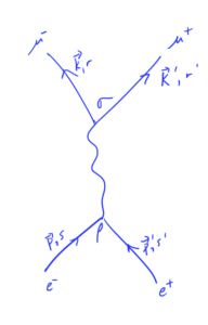
  • Muon pair production

    We then studied muon pair production in detail, and determined the form of the scattering matrix element
    \begin{equation*}
    i M
    =
    i \frac{e^2}{q^2}
    \overline{v}^{s’}(p’) \gamma^\rho u^s(p)
    \overline{u}^r(k) \gamma_\rho v^{r’}(k’),
    \end{equation*}
    where the \( (2 \pi)^4 \delta^4(…) \) term hasn’t been made explicit, and detemined that the average of its square over all input and output polarization (spin) states was
    \begin{equation*}
    \inv{4} \sum_{ss’, rr’} \Abs{M}^2
    =
    \frac{e^4}{4 q^4}
    \textrm{tr}{ \lr{
    \lr{ \gamma^\alpha {k’}_\alpha – m_\mu }
    \gamma_\nu
    \lr{ \gamma^\beta {k}_\beta + m_\mu }
    \gamma_\mu
    }}
    \times
    \textrm{tr}{ \lr{
    \lr{ \gamma^\kappa {p}_\kappa + m_e }
    \gamma^\nu
    \lr{ \gamma^\rho {p’}_\rho – m_e }
    \gamma^\mu
    }}.
    \end{equation*}.
    In the CM frame (neglecting the electron mass, which is small relative to the muon mass), this reduced to
    \begin{equation*}
    \inv{4} \sum_{\text{spins}} \Abs{M}^2
    =
    \frac{8 e^4}{q^4}
    \lr{
    p \cdot k’ p’ \cdot k
    + p \cdot k p’ \cdot k’
    + p \cdot p’ m_\mu^2
    }.
    \end{equation*}

  • We computed the differential cross section
    \begin{equation*}
    {\frac{d\sigma}{d\Omega}}_{\text{CM}}
    =
    \frac{\alpha^2}{4 E_{\text{CM}}^2 }
    \sqrt{ 1 – \frac{m_\mu^2}{E^2} }
    \lr{
    1 + \frac{m_\mu^2}{E^2}
    + \lr{ 1 – \frac{m_\mu^2}{E^2} } \cos^2\theta
    },
    \end{equation*}
    and the total cross section
    \begin{equation*}
    \sigma_{\text{total}}
    =
    \frac{4 \pi \alpha^2}{3 E_{\text{CM}}^2 }
    \sqrt{ 1 – \frac{m_\mu^2}{E^2} }
    \lr{
    1 + \inv{2} \frac{m_\mu^2}{E^2}
    },
    \end{equation*}
    and compared that to the cross section that we was determined with the dimensional analysis handwaving at the start of the course.
  • We finished off with a quick discussion of quark pair production, and how some of the calculations we performed for muon pair production can be used to measure and validate the intermediate quark states that were theorized as carriers of the strong force.

References

[1] Michael E Peskin and Daniel V Schroeder. An introduction to Quantum Field Theory. Westview, 1995.

PHY2403H Quantum Field Theory. Lecture 16: Differential cross section, scattering, pair production, transition amplitude, decay rate, S-matrix, connected and amputated diagrams, vacuum fluctuation, symmetry coefficient. Taught by Prof. Erich Poppitz

November 13, 2018 phy2403 , , , , , , , ,

Here are my [lecture notes from last Wednesday’s class], which are posted out of sequence and only in PDF format this time.

PHY2403H Quantum Field Theory. Lecture 17: Scattering, decay, cross sections in a scalar theory. Taught by Prof. Erich Poppitz

November 12, 2018 phy2403 , , ,

[Click here for a PDF of this post with nicer formatting]

DISCLAIMER: Very rough notes from class (today VERY VERY rough).

These are notes for the UofT course PHY2403H, Quantum Field Theory, taught by Prof. Erich Poppitz, fall 2018.

Review: S-matrix

We defined an \( S-\)matrix
\begin{equation}\label{eqn:qftLecture17:20}
\bra{f} S \ket{i} = S_{fi} = \lr{ 2 \pi }^4 \delta^{(4)} \lr{ \sum \lr{p_i – \sum_{p_f} } } i M_{fi},
\end{equation}
where
\begin{equation}\label{eqn:qftLecture17:40}
i M_{fi} = \sum \text{ all connected amputated Feynman diagrams }.
\end{equation}
The matrix element \( \bra{f} S \ket{i} \) is the amplitude of the transition from the initial to the final state. In general this can get very complicated, as the number of terms grows factorially with the order.

We also talked about decays.

Scattering in a scalar theory

Suppose that we have a scalar theory with a light field \( \Phi, M \) and a heavy field \( \varphi, m \), where \( m > 2 M \). Perhaps we have an interaction with a \( z^2 \) symmetry so that the interaction potential is quadratic in \( \Phi \)
\begin{equation}\label{eqn:qftLecture17:60}
V_{\text{int}} = \mu \varphi \Phi \Phi.
\end{equation}
We may have \( \Phi \Phi \rightarrow \Phi \Phi \) scattering.

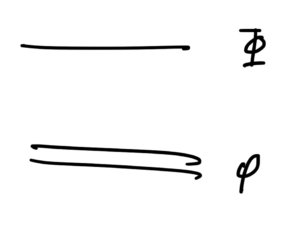
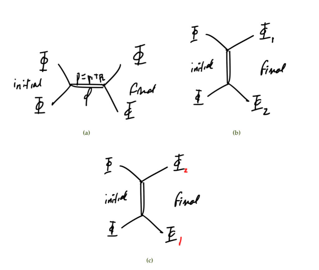
We will denote diagrams using a double line for \( \phi \) and a single line for \( \Phi \), as sketched in

fig. 1. Particle line convention.


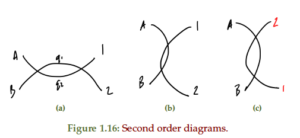
There are three possible diagrams:

fig 2. Possible diagrams.

The first we will call the s-channel, which has amplitude

\begin{equation}\label{eqn:qftLecture17:80}
A(\text{s-channel}) \sim \frac{i}{p^2 – m^2 + i \epsilon} =
\frac{i}{s – m^2 + i \epsilon}
\end{equation}

\begin{equation}\label{eqn:qftLecture17:100}
(p_1 + p_2)^2 = s
\end{equation}
In the centre of mass frame
\begin{equation}\label{eqn:qftLecture17:120}
\Bp_1 = – \Bp_2,
\end{equation}
so
\begin{equation}\label{eqn:qftLecture17:140}
s = \lr{ p_1^0 + p_2^0 }^2 = E_{\text{cm}}^2.
\end{equation}

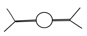
To the next order we have a diagram like fig. 3.

fig. 3. Higher order.

and can have additional virtual particles created, with diagrams like fig. 4.

fig. 4. More virtual particles.


We will see (QFT II) that this leads to an addition imaginary \( i \Gamma \) term in the propagator
\begin{equation}\label{eqn:qftLecture17:160}
\frac{i}{s – m^2 + i \epsilon}
\rightarrow
\frac{i}{s – m^2 – i m \Gamma + i \epsilon}.
\end{equation}
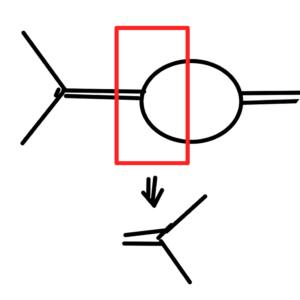
If we choose to zoom into the such a figure, as sketched in fig. 5, we find that it contains the interaction of interest for our diagram, so we can (looking forward to currently unknown material) know that our diagram also has such an imaginary \( i \Gamma \) term in its propagator.

fig. 5. Zooming into the diagram for a higher order virtual particle creation event.

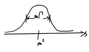
Assuming such a term, the squared amplitude becomes
\begin{equation}\label{eqn:qftLecture17:180}
\evalbar{\sigma}{s \text{near} m^2}
\sim
\Abs{A_s}^2 \sim \inv{(s – m)^2 + m^2 \Gamma^2}
\end{equation}

This is called a resonance (name?), and is sketched in fig. 6.

fig. 6. Resonance.


Where are the poles of the modified propagator?

\begin{equation}\label{eqn:qftLecture17:220}
\frac{i}{s – m^2 – i m \Gamma + i \epsilon}
=
\frac{i}{p_0^2 – \Bp^2 – m^2 – i m \Gamma + i \epsilon}
\end{equation}

The pole is found, neglecting \( i \epsilon \), is found at
\begin{equation}\label{eqn:qftLecture17:200}
\begin{aligned}
p_0
&= \sqrt{ \omega_\Bp^2 + i m \Gamma } \\
&= \omega_\Bp \sqrt{ 1 + \frac{i m \Gamma }{\omega_\Bp^2} } \\
&\approx \omega_\Bp + \frac{i m \Gamma }{2 \omega_\Bp}
\end{aligned}
\end{equation}

Decay rates.

We have an initial state
\begin{equation}\label{eqn:qftLecture17:240}
\ket{i} = \ket{k},
\end{equation}
and final state
\begin{equation}\label{eqn:qftLecture17:260}
\ket{f} = \ket{p_1^f, p_2^f \cdots p_n^f}.
\end{equation}
We defined decay rate as the ratio of the number of initial particles to the number of final particles.

The probability is
\begin{equation}\label{eqn:qftLecture17:280}
\rho \sim \Abs{\bra{f} S \ket{i}}^2
=
(2 \pi)^4 \delta^{(4)}( p_{\text{in}} – \sum p_f )
\times \Abs{ M_{fi} }^2
\end{equation}

Saying that \( \delta(x) f(x) = \delta(x) f(0) \) we can set the argument of one of the delta functions to zero, which gives us a vacuum volume element factor
\begin{equation}\label{eqn:qftLecture17:300}
(2 \pi)^4
\delta^{(4)}( p_{\text{in}} – \sum p_f ) =
(2 \pi)^4
\delta^{(4)}( 0 )
= V_3 T,
\end{equation}
so
\begin{equation}\label{eqn:qftLecture17:320}
\frac{\text{probability for \( i \rightarrow f\)}}{\text{unit time}}
\sim
(2 \pi)^4 \delta^{(4)}( p_{\text{in}} – \sum p_f )
V_3
\times \Abs{ M_{fi} }^2
\end{equation}

\begin{equation}\label{eqn:qftLecture17:340}
\braket{\Bk}{\Bk} = 2 \omega_\Bk V_3
\end{equation}

coming from

\begin{equation}\label{eqn:qftLecture17:360}
\braket{k}{p} = (2 \pi)^3 2 \omega_\Bp \delta^{(3)}(\Bp – \Bk)
\end{equation}
so
\begin{equation}\label{eqn:qftLecture17:380}
\braket{k}{k} = 2 \omega_\Bp V_3
\end{equation}

\begin{equation}\label{eqn:qftLecture17:400}
\frac{\text{probability for \(i \rightarrow f\)}}{\text{unit time}}
\sim
\frac{
(2 \pi)^4 \delta^{(4)}( p_{\text{in}} – \sum p_f )
\Abs{ M_{fi} }^2 V_3
}
{
2 \omega_\Bk V_3
2 \omega_{\Bp_1}
\cdots
2 \omega_{\Bp_n} V_3^n
}
\end{equation}

If we multiply the number of final states with \( p_i^f \in (p_i^f, p_i^f + dp_i^f) \) for a particle in a box
\begin{equation}\label{eqn:qftLecture17:420}
p_x = \frac{ 2 \pi n_x}{L}
\end{equation}

\begin{equation}\label{eqn:qftLecture17:440}
\Delta p_x = \frac{ 2 \pi }{L} \Delta n_x
\end{equation}

\begin{equation}\label{eqn:qftLecture17:460}
\Delta n_x
=
\frac{L}{2 \pi} \Delta p_x
\end{equation}

and

\begin{equation}\label{eqn:qftLecture17:480}
\Delta n_x
\Delta n_y
\Delta n_z
= \frac{V_3}{(2 \pi)^3 }
\Delta p_x
\Delta p_y
\Delta p_z
\end{equation}

\begin{equation}\label{eqn:qftLecture17:500}
\begin{aligned}
\Gamma
&=
\frac{\text{number of events \( i \rightarrow f \)}}{\text{unit time}} \\
&=
\prod_{f} \frac{ d^3 p}{(2 \pi)^3 2 \omega_{\Bp^f} }
\frac{ (2 \pi)^4 \delta^{(4)}( k – \sum_f p^f ) \Abs{M_{fi}}^2 }
{
2 \omega_{\Bk}
}
\end{aligned}
\end{equation}

Note that everything here is Lorentz invariant except for the denominator of the second term ( \(2 \omega_{\Bk}\)). This is a well known result (the decay rate changes in different frames).

Cross section.

For \( 2 \rightarrow \text{many} \) transitions

\begin{equation}\label{eqn:qftLecture17:520}
\frac{\text{probability \( i \rightarrow f \)}}{\text{unit time}}
\times \lr{
\text{ number of final states with \( p_f \in (p_f, p_f + dp_f) \)
}
}
=
\frac{ (2 \pi)^4 \delta^{(4)}( \sum p_i – \sum_f p^f ) \Abs{M_{fi}}^2 {V_3} }
{
2 \omega_{\Bk_1} V_3
2 \omega_{\Bk_2} {V_3 }
}
\prod_{f} \frac{ d^3 p}{(2 \pi)^3 2 \omega_{\Bp^f} }
\end{equation}

We need to divide by the flux.

In the CM frame, as sketched in fig. 7, the current is
\begin{equation}\label{eqn:qftLecture17:540}
\Bj = n \Bv_1 – n \Bv_2,
\end{equation}
so if the density is
\begin{equation}\label{eqn:qftLecture17:560}
n = \inv{V_3},
\end{equation}
(one particle in \(V_3\)), then
\begin{equation}\label{eqn:qftLecture17:580}
\Bj = \frac{\Bv_1 – \Bv_2}{V_3}.
\end{equation}

fig. 7. Centre of mass frame.


This is where [1] stops,
\begin{equation}\label{eqn:qftLecture17:640}
\sigma
=
\frac{ (2 \pi)^4 \delta^{(4)}( \sum p_i – \sum_f p^f ) \Abs{M_{fi}}^2 {V_3} }
{
2 \omega_{\Bk_1}
2 \omega_{\Bk_2}
\Abs{\Bv_1 – \Bv_2}
}
\prod_{f} \frac{ d^3 p}{(2 \pi)^3 2 \omega_{\Bp^f} }
\end{equation}

There is, however, a nice Lorentz invariant generalization
\begin{equation}\label{eqn:qftLecture17:600}
j = \inv{ V_3 \omega_{k_A} \omega_{k_B}} \sqrt{ (k_A – k_B)^2 – m_A^2 m_B^2 }
\end{equation}

(Claim: DIY)
\begin{equation}\label{eqn:qftLecture17:620}
\begin{aligned}
\evalbar{j}{CM}
&=
\inv{V_3}
\lr{
\frac{\Abs{\Bk}}{\omega_{k_A}}
+
\frac{\Abs{\Bk}}{\omega_{k_B}}
} \\
&=
\inv{V_3} \lr{ \Abs{\Bv_A} + \Abs{\Bv_B} } \\
&=
\inv{V_3} \Abs{\Bv_1 – \Bv_2 }.
\end{aligned}
\end{equation}

\begin{equation}\label{eqn:qftLecture17:660}
\sigma
=
\frac{ (2 \pi)^4 \delta^{(4)}( \sum p_i – \sum_f p^f ) \Abs{M_{fi}}^2 {V_3} }
{
4 \sqrt{ (k_A – k_B)^2 – m_A^2 m_B^2 }
}
\prod_{f} \frac{ d^3 p}{(2 \pi)^3 2 \omega_{\Bp^f} }.
\end{equation}

References

[1] Michael E Peskin and Daniel V Schroeder. An introduction to Quantum Field Theory. Westview, 1995.

PHY2403H Quantum Field Theory. Lecture 15b: Wick’s theorem, vacuum expectation, Feynman diagrams, phi^4 interaction, tree level diagrams, scattering, cross section, differential cross section. Taught by Prof. Erich Poppitz

November 7, 2018 phy2403 , , , , , , ,

[Here are my notes for the second half of last wednesday’s lecture]. Because the simplewick latex package is required to format these meaningfully, and that’s not available in wordpress latex, I’m not going to attempt to make a web viewable version in addition to the pdf.