[If mathjax doesn’t display properly for you, click here for a PDF of this post]
Motivation.
I started pondering some aspects of spacetime integration theory, and found that there were some aspects of the concepts of reciprocal frames that were not clear to me. In the process of sorting those ideas out for myself, I wrote up the following notes.
In the notes below, I will introduce the many of the prerequisite ideas that are needed to express and apply the fundamental theorem of geometric calculus in a 4D relativistic context. The focus will be the Dirac’s algebra of special relativity, known as STA (Space Time Algebra) in geometric algebra parlance. If desired, it should be clear how to apply these ideas to lower or higher dimensional spaces, and to plain old Euclidean metrics.
On notation.
In Euclidean space we use bold face reciprocal frame vectors \( \Bx^i \cdot \Bx_j = {\delta^i}_j \), which nicely distinguishes them from the generalized coordinates \( x_i, x^j \) associated with the basis or the reciprocal frame, that is
\begin{equation}\label{eqn:reciprocalblog:640}
\Bx = x^i \Bx_i = x_j \Bx^j.
\end{equation}
On the other hand, it is conventional to use non-bold face for both the four-vectors and their coordinates in STA, such as the following standard basis decomposition
\begin{equation}\label{eqn:reciprocalblog:660}
x = x^\mu \gamma_\mu = x_\mu \gamma^\mu.
\end{equation}
If we use non-bold face \( x^\mu, x_\nu \) for the coordinates with respect to a specified frame, then we cannot also use non-bold face for the curvilinear basis vectors.
To resolve this notational ambiguity, I’ve chosen to use bold face \( \Bx^\mu, \Bx_\nu \) symbols as the curvilinear basis elements in this relativistic context, as we do for Euclidean spaces.
Basis and coordinates.
Definition 1.1: Standard Dirac basis.
The Dirac basis elements are \(\setlr{ \gamma_0, \gamma_1, \gamma_2, \gamma_3 } \), satisfying
\begin{equation}\label{eqn:reciprocalblog:1940}
\gamma_0^2 = 1 = -\gamma_k^2, \quad \forall k = 1,2,3,
\end{equation}
and
\begin{equation}\label{eqn:reciprocalblog:740}
\gamma_\mu \cdot \gamma_\nu = 0, \quad \forall \mu \ne \nu.
\end{equation}
A conventional way of summarizing these orthogonality relationships is \( \gamma_\mu \cdot \gamma_\nu = \eta_{\mu\nu} \), where \( \eta_{\mu\nu} \) are the elements of the metric \( G = \text{diag}(+,-,-,-) \).
Definition 1.2: Reciprocal basis for the standard Dirac basis.
We define a reciprocal basis \( \setlr{ \gamma^0, \gamma^1, \gamma^2, \gamma^3} \) satisfying \( \gamma^\mu \cdot \gamma_\nu = {\delta^\mu}_\nu, \forall \mu,\nu \in 0,1,2,3 \).
Theorem 1.1: Reciprocal basis uniqueness.
This reciprocal basis is unique, and for our choice of metric has the values
\begin{equation}\label{eqn:reciprocalblog:1960}
\gamma^0 = \gamma_0, \quad \gamma^k = -\gamma_k, \quad \forall k = 1,2,3.
\end{equation}
Proof is left to the reader.
Definition 1.3: Coordinates.
We define the coordinates of a vector with respect to the standard basis as \( x^\mu \) satisfying
\begin{equation}\label{eqn:reciprocalblog:1980}
x = x^\mu \gamma_\mu,
\end{equation}
and define the coordinates of a vector with respect to the reciprocal basis as \( x_\mu \) satisfying
\begin{equation}\label{eqn:reciprocalblog:2000}
x = x_\mu \gamma^\mu,
\end{equation}
Theorem 1.2: Coordinates.
Given the definitions above, we may compute the coordinates of a vector, simply by dotting with the basis elements
\begin{equation}\label{eqn:reciprocalblog:2020}
x^\mu = x \cdot \gamma^\mu,
\end{equation}
and
\begin{equation}\label{eqn:reciprocalblog:2040}
x_\mu = x \cdot \gamma_\mu,
\end{equation}
Start proof:
This follows by straightforward computation
\begin{equation}\label{eqn:reciprocalblog:840}
\begin{aligned}
x \cdot \gamma^\mu
&=
\lr{ x^\nu \gamma_\nu } \cdot \gamma^\mu \\
&=
x^\nu \lr{ \gamma_\nu \cdot \gamma^\mu } \\
&=
x^\nu {\delta_\nu}^\mu \\
&=
x^\mu,
\end{aligned}
\end{equation}
and
\begin{equation}\label{eqn:reciprocalblog:860}
\begin{aligned}
x \cdot \gamma_\mu
&=
\lr{ x_\nu \gamma^\nu } \cdot \gamma_\mu \\
&=
x_\nu \lr{ \gamma^\nu \cdot \gamma_\mu } \\
&=
x_\nu {\delta^\nu}_\mu \\
&=
x_\mu.
\end{aligned}
\end{equation}
End proof.
Derivative operators.
We’d like to determine the form of the (spacetime) gradient operator. The gradient can be defined in terms of coordinates directly, but we choose an implicit definition, in terms of the directional derivative.
Definition 1.4: Directional derivative and gradient.
Let \( F = F(x) \) be a four-vector parameterized multivector. The directional derivative of \( F \) with respect to the (four-vector) direction \( a \) is denoted
\begin{equation}\label{eqn:reciprocalblog:2060}
\lr{ a \cdot \grad } F = \lim_{\epsilon \rightarrow 0} \frac{ F(x + \epsilon a) – F(x) }{ \epsilon },
\end{equation}
where \( \grad \) is called the space time gradient.
Theorem 1.3: Gradient.
The standard basis representation of the gradient is
\begin{equation}\label{eqn:reciprocalblog:2080}
\grad = \gamma^\mu \partial_\mu,
\end{equation}
where
\begin{equation}\label{eqn:reciprocalblog:2100}
\partial_\mu = \PD{x^\mu}{}.
\end{equation}
Start proof:
The Dirac gradient pops naturally out of the coordinate representation of the directional derivative, as we can see by expanding \( F(x + \epsilon a) \) in Taylor series
\begin{equation}\label{eqn:reciprocalblog:900}
\begin{aligned}
F(x + \epsilon a)
&= F(x) + \epsilon \frac{dF(x + \epsilon a)}{d\epsilon} + O(\epsilon^2) \\
&= F(x) + \epsilon \PD{\lr{x^\mu + \epsilon a^\mu}}{F} \PD{\epsilon}{\lr{x^\mu + \epsilon a^\mu}} \\
&= F(x) + \epsilon \PD{\lr{x^\mu + \epsilon a^\mu}}{F} a^\mu.
\end{aligned}
\end{equation}
The directional derivative is
\begin{equation}\label{eqn:reciprocalblog:920}
\begin{aligned}
\lim_{\epsilon \rightarrow 0}
\frac{F(x + \epsilon a) – F(x)}{\epsilon}
&=
\lim_{\epsilon \rightarrow 0}\,
a^\mu
\PD{\lr{x^\mu + \epsilon a^\mu}}{F} \\
&=
a^\mu
\PD{x^\mu}{F} \\
&=
\lr{a^\nu \gamma_\nu} \cdot \gamma^\mu \PD{x^\mu}{F} \\
&=
a \cdot \lr{ \gamma^\mu \partial_\mu } F.
\end{aligned}
\end{equation}
End proof.
Curvilinear bases.
Curvilinear bases are the foundation of the fundamental theorem of multivector calculus. This form of integral calculus is defined over parameterized surfaces (called manifolds) that satisfy some specific non-degeneracy and continuity requirements.
A parameterized vector \( x(u,v, \cdots w) \) can be thought of as tracing out a hypersurface (curve, surface, volume, …), where the dimension of the hypersurface depends on the number of parameters. At each point, a bases can be constructed from the differentials of the parameterized vector. Such a basis is called the tangent space to the surface at the point in question. Our curvilinear bases will be related to these differentials. We will also be interested in a dual basis that is restricted to the span of the tangent space. This dual basis will be called the reciprocal frame, and line the basis of the tangent space itself, also varies from point to point on the surface.

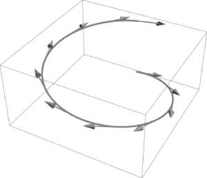
Fig 1a. One parameter curve, with illustration of tangent space along the curve.

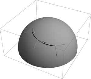
Fig 1b. Two parameter surface, with illustration of tangent space along the surface.
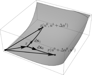
One and two parameter spaces are illustrated in fig. 1a, and 1b. The tangent space basis at a specific point of a two parameter surface, \( x(u^0, u^1) \), is illustrated in fig. 1. The differential directions that span the tangent space are
\begin{equation}\label{eqn:reciprocalblog:1040}
\begin{aligned}
d\Bx_0 &= \PD{u^0}{x} du^0 \\
d\Bx_1 &= \PD{u^1}{x} du^1,
\end{aligned}
\end{equation}
and the tangent space itself is \( \mbox{Span}\setlr{ d\Bx_0, d\Bx_1 } \). We may form an oriented surface area element \( d\Bx_0 \wedge d\Bx_1 \) over this surface.

Fig 2. Two parameter surface.
Tangent spaces associated with 3 or more parameters cannot be easily visualized in three dimensions, but the idea generalizes algebraically without trouble.
Definition 1.5: Tangent basis and space.
Given a parameterization \( x = x(u^0, \cdots, u^N) \), where \( N < 4 \), the span of the vectors
\begin{equation}\label{eqn:reciprocalblog:2120}
\Bx_\mu = \PD{u^\mu}{x},
\end{equation}
is called the tangent space for the hypersurface associated with the parameterization, and it’s basis is
\( \setlr{ \Bx_\mu } \).
Later we will see that parameterization constraints must be imposed, as not all surfaces generated by a set of parameterizations are useful for integration theory. In particular, degenerate parameterizations for which the wedge products of the tangent space basis vectors are zero, or those wedge products cannot be inverted, are not physically meaningful. Properly behaved surfaces of this sort are called manifolds.
Having introduced curvilinear coordinates associated with a parameterization, we can now determine the form of the gradient with respect to a parameterization of spacetime.
Theorem 1.4: Gradient, curvilinear representation.
Given a spacetime parameterization \( x = x(u^0, u^1, u^2, u^3) \), the gradient with respect to the parameters \( u^\mu \) is
\begin{equation}\label{eqn:reciprocalblog:2140}
\grad = \sum_\mu \Bx^\mu
\PD{u^\mu}{},
\end{equation}
where
\begin{equation}\label{eqn:reciprocalblog:2160}
\Bx^\mu = \grad u^\mu.
\end{equation}
The vectors \( \Bx^\mu \) are called the reciprocal frame vectors, and the ordered set \( \setlr{ \Bx^0, \Bx^1, \Bx^2, \Bx^3 } \) is called the reciprocal basis.It is convenient to define \( \partial_\mu \equiv \PDi{u^\mu}{} \), so that the gradient can be expressed in mixed index representation
\begin{equation}\label{eqn:reciprocalblog:2180}
\grad = \Bx^\mu \partial_\mu.
\end{equation}
This introduces some notational ambiguity, since we used \( \partial_\mu = \PDi{x^\mu}{} \) for the standard basis derivative operators too, but we will be careful to be explicit when there is any doubt about what is intended.
Start proof:
The proof follows by application of the chain rule.
\begin{equation}\label{eqn:reciprocalblog:960}
\begin{aligned}
\grad F
&=
\gamma^\alpha \PD{x^\alpha}{F} \\
&=
\gamma^\alpha
\PD{x^\alpha}{u^\mu}
\PD{u^\mu}{F} \\
&=
\lr{ \grad u^\mu } \PD{u^\mu}{F} \\
&=
\Bx^\mu \PD{u^\mu}{F}.
\end{aligned}
\end{equation}
End proof.
Theorem 1.5: Reciprocal relationship.
The vectors \( \Bx^\mu = \grad u^\mu \), and \( \Bx_\mu = \PDi{u^\mu}{x} \) satisfy the reciprocal relationship
\begin{equation}\label{eqn:reciprocalblog:2200}
\Bx^\mu \cdot \Bx_\nu = {\delta^\mu}_\nu.
\end{equation}
Start proof:
\begin{equation}\label{eqn:reciprocalblog:1020}
\begin{aligned}
\Bx^\mu \cdot \Bx_\nu
&=
\grad u^\mu \cdot
\PD{u^\nu}{x} \\
&=
\lr{
\gamma^\alpha \PD{x^\alpha}{u^\mu}
}
\cdot
\lr{
\PD{u^\nu}{x^\beta} \gamma_\beta
} \\
&=
{\delta^\alpha}_\beta \PD{x^\alpha}{u^\mu}
\PD{u^\nu}{x^\beta} \\
&=
\PD{x^\alpha}{u^\mu} \PD{u^\nu}{x^\alpha} \\
&=
\PD{u^\nu}{u^\mu} \\
&=
{\delta^\mu}_\nu
.
\end{aligned}
\end{equation}
End proof.
It is instructive to consider an example. Here is a parameterization that scales the proper time parameter, and uses polar coordinates in the \(x-y\) plane.
Problem: Compute the curvilinear and reciprocal basis.
Given
\begin{equation}\label{eqn:reciprocalblog:2360}
x(t,\rho,\theta,z) = c t \gamma_0 + \gamma_1 \rho e^{i \theta} + z \gamma_3,
\end{equation}
where \( i = \gamma_1 \gamma_2 \), compute the curvilinear frame vectors and their reciprocals.
Answer
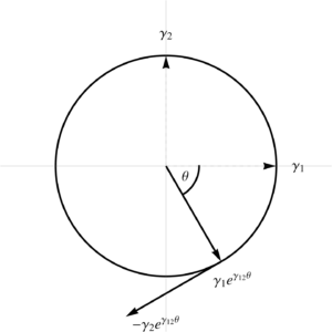
The frame vectors are all easy to compute
\begin{equation}\label{eqn:reciprocalblog:1180}
\begin{aligned}
\Bx_0 &= \PD{t}{x} = c \gamma_0 \\
\Bx_1 &= \PD{\rho}{x} = \gamma_1 e^{i \theta} \\
\Bx_2 &= \PD{\theta}{x} = \rho \gamma_1 \gamma_1 \gamma_2 e^{i \theta} = – \rho \gamma_2 e^{i \theta} \\
\Bx_3 &= \PD{z}{x} = \gamma_3.
\end{aligned}
\end{equation}
The \( \Bx_1 \) vector is radial, \( \Bx^2 \) is perpendicular to that tangent to the same unit circle, as plotted in fig 3.

Fig3: Tangent space direction vectors.
All of these particular frame vectors happen to be mutually perpendicular, something that will not generally be true for a more arbitrary parameterization.
To compute the reciprocal frame vectors, we must express our parameters in terms of \( x^\mu \) coordinates, and use implicit integration techniques to deal with the coupling of the rotational terms. First observe that
\begin{equation}\label{eqn:reciprocalblog:1200}
\gamma_1 e^{i\theta}
= \gamma_1 \lr{ \cos\theta + \gamma_1 \gamma_2 \sin\theta }
= \gamma_1 \cos\theta – \gamma_2 \sin\theta,
\end{equation}
so
\begin{equation}\label{eqn:reciprocalblog:1220}
\begin{aligned}
x^0 &= c t \\
x^1 &= \rho \cos\theta \\
x^2 &= -\rho \sin\theta \\
x^3 &= z.
\end{aligned}
\end{equation}
We can easily evaluate the \( t, z \) gradients
\begin{equation}\label{eqn:reciprocalblog:1240}
\begin{aligned}
\grad t &= \frac{\gamma^1 }{c} \\
\grad z &= \gamma^3,
\end{aligned}
\end{equation}
but the \( \rho, \theta \) gradients are not as easy. First writing
\begin{equation}\label{eqn:reciprocalblog:1260}
\rho^2 = \lr{x^1}^2 + \lr{x^2}^2,
\end{equation}
we find
\begin{equation}\label{eqn:reciprocalblog:1280}
\begin{aligned}
2 \rho \grad \rho = 2 \lr{ x^1 \grad x^1 + x^2 \grad x^2 }
&= 2 \rho \lr{ \cos\theta \gamma^1 – \sin\theta \gamma^2 } \\
&= 2 \rho \gamma^1 \lr{ \cos\theta – \gamma_1 \gamma^2 \sin\theta } \\
&= 2 \rho \gamma^1 e^{i\theta},
\end{aligned}
\end{equation}
so
\begin{equation}\label{eqn:reciprocalblog:1300}
\grad \rho = \gamma^1 e^{i\theta}.
\end{equation}
For the \( \theta \) gradient, we can write
\begin{equation}\label{eqn:reciprocalblog:1320}
\tan\theta = -\frac{x^2}{x^1},
\end{equation}
so
\begin{equation}\label{eqn:reciprocalblog:1340}
\begin{aligned}
\inv{\cos^2 \theta} \grad \theta
&= -\frac{\gamma^2}{x^1} – x^2 \frac{-\gamma^1}{\lr{x^1}^2} \\
&= \inv{\lr{x^1}^2} \lr{ – \gamma^2 x^1 + \gamma^1 x^2 } \\
&= \frac{\rho}{\rho^2 \cos^2\theta } \lr{ – \gamma^2 \cos\theta – \gamma^1 \sin\theta } \\
&= -\frac{1}{\rho \cos^2\theta } \gamma^2 \lr{ \cos\theta + \gamma_2 \gamma^1 \sin\theta } \\
&= -\frac{\gamma^2 e^{i\theta} }{\rho \cos^2\theta },
\end{aligned}
\end{equation}
or
\begin{equation}\label{eqn:reciprocalblog:1360}
\grad\theta = -\inv{\rho} \gamma^2 e^{i\theta}.
\end{equation}
In summary,
\begin{equation}\label{eqn:reciprocalblog:1380}
\begin{aligned}
\Bx^0 &= \frac{\gamma^0}{c} \\
\Bx^1 &= \gamma^1 e^{i\theta} \\
\Bx^2 &= -\inv{\rho} \gamma^2 e^{i\theta} \\
\Bx^3 &= \gamma^3.
\end{aligned}
\end{equation}
Despite being a fairly simple parameterization, it was still fairly difficult to solve for the gradients when the parameterization introduced coupling between the coordinates. In this particular case, we could have solved for the parameters in terms of the coordinates (but it was easier not to), but that will not generally be true. We want a less labor intensive strategy to find the reciprocal frame. When we have a full parameterization of spacetime, then we can do this with nothing more than a matrix inversion.
Theorem 1.6: Reciprocal frame matrix equations.
Given a spacetime basis \( \setlr{\Bx_0, \cdots \Bx_3} \), let \( [\Bx_\mu] \) and \( [\Bx^\nu] \) be column matrices with the coordinates of these vectors and their reciprocals, with respect to the standard basis \( \setlr{\gamma_0, \gamma_1, \gamma_2, \gamma_3 } \). Let
\begin{equation}\label{eqn:reciprocalblog:2220}
A =
\begin{bmatrix}
[\Bx_0] & \cdots & [\Bx_{3}]
\end{bmatrix}
,\qquad
X =
\begin{bmatrix}
[\Bx^0] & \cdots & [\Bx^{3}]
\end{bmatrix}.
\end{equation}
The coordinates of the reciprocal frame vectors can be found by solving
\begin{equation}\label{eqn:reciprocalblog:2240}
A^\T G X = 1,
\end{equation}
where \( G = \text{diag}(1,-1,-1,-1) \) and the RHS is an \( 4 \times 4 \) identity matrix.
Start proof:
Let \( \Bx_\mu = {a_\mu}^\alpha \gamma_\alpha, \Bx^\nu = b^{\nu\beta} \gamma_\beta \), so that
\begin{equation}\label{eqn:reciprocalblog:140}
A =
\begin{bmatrix}
{a_\nu}^\mu
\end{bmatrix},
\end{equation}
and
\begin{equation}\label{eqn:reciprocalblog:160}
X =
\begin{bmatrix}
b^{\nu\mu}
\end{bmatrix},
\end{equation}
where \( \mu \in [0,3]\) are the row indexes and \( \nu \in [0,N-1]\) are the column indexes. The reciprocal frame satisfies \( \Bx_\mu \cdot \Bx^\nu = {\delta_\mu}^\nu \), which has the coordinate representation of
\begin{equation}\label{eqn:reciprocalblog:180}
\begin{aligned}
\Bx_\mu \cdot \Bx^\nu
&=
\lr{
{a_\mu}^\alpha \gamma_\alpha
}
\cdot
\lr{
b^{\nu\beta} \gamma_\beta
} \\
&=
{a_\mu}^\alpha
\eta_{\alpha\beta}
b^{\nu\beta} \\
&=
{[A^\T G B]_\mu}^\nu,
\end{aligned}
\end{equation}
where \( \mu \) is the row index and \( \nu \) is the column index.
End proof.
Problem: Matrix inversion reciprocals.
For the parameterization of \ref{eqn:reciprocalblog:2360}, find the reciprocal frame vectors by matrix inversion.
Answer
We expanded \( \Bx_1 \) explicitly in \ref{eqn:reciprocalblog:1200}. Doing the same for \( \Bx_2 \), we have
\begin{equation}\label{eqn:reciprocalblog:1201}
\Bx_2 =
-\rho \gamma_2 e^{i\theta}
= -\rho \gamma_2 \lr{ \cos\theta + \gamma_1 \gamma_2 \sin\theta }
= – \rho \lr{ \gamma_2 \cos\theta + \gamma_1 \sin\theta}.
\end{equation}
Reading off the coordinates of our frame vectors, we have
\begin{equation}\label{eqn:reciprocalblog:1400}
X =
\begin{bmatrix}
c & 0 & 0 & 0 \\
0 & C & -\rho S & 0 \\
0 & -S & -\rho C & 0 \\
0 & 0 & 0 & 1 \\
\end{bmatrix},
\end{equation}
where \( C = \cos\theta \) and \( S = \sin\theta \). We want
\begin{equation}\label{eqn:reciprocalblog:1420}
Y =
{\begin{bmatrix}
c & 0 & 0 & 0 \\
0 & -C & S & 0 \\
0 & \rho S & \rho C & 0 \\
0 & 0 & 0 & -1 \\
\end{bmatrix}}^{-1}
=
\begin{bmatrix}
\inv{c} & 0 & 0 & 0 \\
0 & -C & \frac{S}{\rho} & 0 \\
0 & S & \frac{C}{\rho} & 0 \\
0 & 0 & 0 & -1 \\
\end{bmatrix}.
\end{equation}
We can read off the coordinates of the reciprocal frame vectors
\begin{equation}\label{eqn:reciprocalblog:1440}
\begin{aligned}
\Bx^0 &= \inv{c} \gamma_0 \\
\Bx^1 &= -\cos\theta \gamma_1 + \sin\theta \gamma_2 \\
\Bx^2 &= \inv{\rho} \lr{ \sin\theta \gamma_1 + \cos\theta \gamma_2 } \\
\Bx^3 &= -\gamma_3.
\end{aligned}
\end{equation}
Factoring out \( \gamma^1 \) from the \( \Bx^1 \) terms, we find
\begin{equation}\label{eqn:reciprocalblog:1460}
\begin{aligned}
\Bx^1
&= -\cos\theta \gamma_1 + \sin\theta \gamma_2 \\
&= \gamma^1 \lr{ \cos\theta + \gamma_1 \gamma_2 \sin\theta } \\
&= \gamma^1 e^{i\theta}.
\end{aligned}
\end{equation}
Similarly for \( \Bx^2 \),
\begin{equation}\label{eqn:reciprocalblog:1480}
\begin{aligned}
\Bx^2
&= \inv{\rho} \lr{ \sin\theta \gamma_1 + \cos\theta \gamma_2 } \\
&= \frac{\gamma^2}{\rho} \lr{ \sin\theta \gamma_2 \gamma_1 – \cos\theta } \\
&= -\frac{\gamma^2}{\rho} e^{i\theta}.
\end{aligned}
\end{equation}
This matches \ref{eqn:reciprocalblog:1380}, as expected, but required only algebraic work to compute.
There will be circumstances where we parameterize only a subset of spacetime, and are interested in calculating quantities associated with such a surface. For example, suppose that
\begin{equation}\label{eqn:reciprocalblog:1500}
x(\rho,\theta) = \gamma_1 \rho e^{i \theta},
\end{equation}
where \( i = \gamma_1 \gamma_2 \) as before. We are now parameterizing only the \(x-y\) plane. We will still find
\begin{equation}\label{eqn:reciprocalblog:1520}
\begin{aligned}
\Bx_1 &= \gamma_1 e^{i \theta} \\
\Bx_2 &= -\gamma_2 \rho e^{i \theta}.
\end{aligned}
\end{equation}
We can compute the reciprocals of these vectors using the gradient method. It’s possible to state matrix equations representing the reciprocal relationship of \ref{eqn:reciprocalblog:2200}, which, in this case, is \( X^\T G Y = 1 \), where the RHS is a \( 2 \times 2 \) identity matrix, and \( X, Y\) are \( 4\times 2\) matrices of coordinates, with
\begin{equation}\label{eqn:reciprocalblog:1540}
X =
\begin{bmatrix}
0 & 0 \\
C & -\rho S \\
-S & -\rho C \\
0 & 0
\end{bmatrix}.
\end{equation}
We no longer have a square matrix problem to solve, and our solution set is multivalued. In particular, this matrix equation has solutions
\begin{equation}\label{eqn:reciprocalblog:1560}
\begin{aligned}
\Bx^1 &= \gamma^1 e^{i\theta} + \alpha \gamma^0 + \beta \gamma^3 \\
\Bx^2 &= -\frac{\gamma^2}{\rho} e^{i\theta} + \alpha’ \gamma^0 + \beta’ \gamma^3.
\end{aligned}
\end{equation}
where \( \alpha, \alpha’, \beta, \beta’ \) are arbitrary constants. In the example we considered, we saw that our \( \rho, \theta \) parameters were functions of only \( x^1, x^2 \), so taking gradients could not introduce any \( \gamma^0, \gamma^3 \) dependence in \( \Bx^1, \Bx^2 \). It seems reasonable to assert that we seek an algebraic method of computing a set of vectors that satisfies the reciprocal relationships, where that set of vectors is restricted to the tangent space. We will need to figure out how to prove that this reciprocal construction is identical to the parameter gradients, but let’s start with figuring out what such a tangent space restricted solution looks like.
Theorem 1.7: Reciprocal frame for two parameter subspace.
Given two vectors, \( \Bx_1, \Bx_2 \), the vectors \( \Bx^1, \Bx^2 \in \mbox{Span}\setlr{ \Bx_1, \Bx_2 } \) such that \( \Bx^\mu \cdot \Bx_\nu = {\delta^\mu}_\nu \) are given by
\begin{equation}\label{eqn:reciprocalblog:2260}
\begin{aligned}
\Bx^1 &= \Bx_2 \cdot \inv{\Bx_1 \wedge \Bx_2} \\
\Bx^2 &= -\Bx_1 \cdot \inv{\Bx_1 \wedge \Bx_2},
\end{aligned}
\end{equation}
provided \( \Bx_1 \wedge \Bx_2 \ne 0 \) and
\( \lr{ \Bx_1 \wedge \Bx_2 }^2 \ne 0 \).
Start proof:
The most general set of vectors that satisfy the span constraint are
\begin{equation}\label{eqn:reciprocalblog:1580}
\begin{aligned}
\Bx^1 &= a \Bx_1 + b \Bx_2 \\
\Bx^2 &= c \Bx_1 + d \Bx_2.
\end{aligned}
\end{equation}
We can use wedge products with either \( \Bx_1 \) or \( \Bx_2 \) to eliminate the other from the RHS
\begin{equation}\label{eqn:reciprocalblog:1600}
\begin{aligned}
\Bx^1 \wedge \Bx_2 &= a \lr{ \Bx_1 \wedge \Bx_2 } \\
\Bx^1 \wedge \Bx_1 &= – b \lr{ \Bx_1 \wedge \Bx_2 } \\
\Bx^2 \wedge \Bx_2 &= c \lr{ \Bx_1 \wedge \Bx_2 } \\
\Bx^2 \wedge \Bx_1 &= – d \lr{ \Bx_1 \wedge \Bx_2 },
\end{aligned}
\end{equation}
and then dot both sides with \( \Bx_1 \wedge \Bx_2 \) to produce four scalar equations
\begin{equation}\label{eqn:reciprocalblog:1640}
\begin{aligned}
a \lr{ \Bx_1 \wedge \Bx_2 }^2
&= \lr{ \Bx^1 \wedge \Bx_2 } \cdot \lr{ \Bx_1 \wedge \Bx_2 } \\
&=
\lr{ \Bx_2 \cdot \Bx_1 } \lr{ \Bx^1 \cdot \Bx_2 }
–
\lr{ \Bx_2 \cdot \Bx_2 } \lr{ \Bx^1 \cdot \Bx_1 } \\
&=
\lr{ \Bx_2 \cdot \Bx_1 } (0)
–
\lr{ \Bx_2 \cdot \Bx_2 } (1) \\
&= – \Bx_2 \cdot \Bx_2
\end{aligned}
\end{equation}
\begin{equation}\label{eqn:reciprocalblog:1660}
\begin{aligned}
– b \lr{ \Bx_1 \wedge \Bx_2 }^2
&=
\lr{ \Bx^1 \wedge \Bx_1 } \cdot \lr{ \Bx_1 \wedge \Bx_2 } \\
&=
\lr{ \Bx^1 \cdot \Bx_2 } \lr{ \Bx_1 \cdot \Bx_1 }
–
\lr{ \Bx^1 \cdot \Bx_1 } \lr{ \Bx_1 \cdot \Bx_2 } \\
&=
(0) \lr{ \Bx_1 \cdot \Bx_1 }
–
(1) \lr{ \Bx_1 \cdot \Bx_2 } \\
&= – \Bx_1 \cdot \Bx_2
\end{aligned}
\end{equation}
\begin{equation}\label{eqn:reciprocalblog:1680}
\begin{aligned}
c \lr{ \Bx_1 \wedge \Bx_2 }^2
&= \lr{ \Bx^2 \wedge \Bx_2 } \cdot \lr{ \Bx_1 \wedge \Bx_2 } \\
&=
\lr{ \Bx_2 \cdot \Bx_1 } \lr{ \Bx^2 \cdot \Bx_2 }
–
\lr{ \Bx_2 \cdot \Bx_2 } \lr{ \Bx^2 \cdot \Bx_1 } \\
&=
\lr{ \Bx_2 \cdot \Bx_1 } (1)
–
\lr{ \Bx_2 \cdot \Bx_2 } (0) \\
&= \Bx_2 \cdot \Bx_1
\end{aligned}
\end{equation}
\begin{equation}\label{eqn:reciprocalblog:1700}
\begin{aligned}
– d \lr{ \Bx_1 \wedge \Bx_2 }^2
&= \lr{ \Bx^2 \wedge \Bx_1 } \cdot \lr{ \Bx_1 \wedge \Bx_2 } \\
&=
\lr{ \Bx_1 \cdot \Bx_1 } \lr{ \Bx^2 \cdot \Bx_2 }
–
\lr{ \Bx_1 \cdot \Bx_2 } \lr{ \Bx^2 \cdot \Bx_1 } \\
&=
\lr{ \Bx_1 \cdot \Bx_1 } (1)
–
\lr{ \Bx_1 \cdot \Bx_2 } (0) \\
&= \Bx_1 \cdot \Bx_1.
\end{aligned}
\end{equation}
Putting the pieces together we have
\begin{equation}\label{eqn:reciprocalblog:1740}
\begin{aligned}
\Bx^1
&= \frac{ – \lr{ \Bx_2 \cdot \Bx_2 } \Bx_1 + \lr{ \Bx_1 \cdot \Bx_2 } \Bx_2
}{\lr{\Bx_1 \wedge \Bx_2}^2} \\
&=
\frac{
\Bx_2 \cdot \lr{ \Bx_1 \wedge \Bx_2 }
}{\lr{\Bx_1 \wedge \Bx_2}^2} \\
&=
\Bx_2 \cdot \inv{\Bx_1 \wedge \Bx_2}
\end{aligned}
\end{equation}
\begin{equation}\label{eqn:reciprocalblog:1760}
\begin{aligned}
\Bx^2
&=
\frac{ \lr{ \Bx_1 \cdot \Bx_2 } \Bx_1 – \lr{ \Bx_1 \cdot \Bx_1 } \Bx_2
}{\lr{\Bx_1 \wedge \Bx_2}^2} \\
&=
\frac{ -\Bx_1 \cdot \lr{ \Bx_1 \wedge \Bx_2 } }
{\lr{\Bx_1 \wedge \Bx_2}^2} \\
&=
-\Bx_1 \cdot \inv{\Bx_1 \wedge \Bx_2}
\end{aligned}
\end{equation}
End proof.
Lemma 1.1: Distribution identity.
Given k-vectors \( B, C \) and a vector \( a \), where the grade of \( C \) is greater than that of \( B \), then
\begin{equation}\label{eqn:reciprocalblog:2280}
\lr{a \wedge B} \cdot C = a \cdot \lr{ B \cdot C }.
\end{equation}
See [1] for a proof.
Theorem 1.8: Higher order tangent space reciprocals.
Given an \(N\) parameter tangent space with basis \( \setlr{ \Bx_0, \Bx_1, \cdots \Bx_{N-1} } \), the reciprocals are given by
\begin{equation}\label{eqn:reciprocalblog:2300}
\Bx^\mu = (-1)^\mu
\lr{ \Bx_0 \wedge \cdots \check{\Bx_\mu} \cdots \wedge \Bx_{N-1} } \cdot I_N^{-1},
\end{equation}
where the checked term (\(\check{\Bx_\mu}\)) indicates that all terms are included in the wedges except the \( \Bx_\mu \) term, and \( I_N = \Bx_0 \wedge \cdots \Bx_{N-1} \) is the pseudoscalar for the tangent space.
Start proof:
I’ll outline the proof for the three parameter tangent space case, from which the pattern will be clear. The motivation for this proof is a reexamination of the algebraic structure of the two vector solution. Suppose we have a tangent space basis \( \setlr{\Bx_0, \Bx_1} \), for which we’ve shown that
\begin{equation}\label{eqn:reciprocalblog:1860}
\begin{aligned}
\Bx^0
&= \Bx_1 \cdot \inv{\Bx_0 \wedge \Bx_1} \\
&= \frac{\Bx_1 \cdot \lr{\Bx_0 \wedge \Bx_1} }{\lr{ \Bx_0 \wedge \Bx_1}^2 }.
\end{aligned}
\end{equation}
If we dot with \( \Bx_0 \) and \( \Bx_1 \) respectively, we find
\begin{equation}\label{eqn:reciprocalblog:1800}
\begin{aligned}
\Bx_0 \cdot \Bx^0
&=
\Bx_0 \cdot \frac{ \Bx_1 \cdot \lr{ \Bx_0 \wedge \Bx_1 } }{\lr{ \Bx_0 \wedge \Bx_1}^2 } \\
&=
\lr{ \Bx_0 \wedge \Bx_1 } \cdot \frac{ \Bx_0 \wedge \Bx_1 }{\lr{ \Bx_0 \wedge \Bx_1}^2 }.
\end{aligned}
\end{equation}
We end up with unity as expected. Here the
“factored” out vector is reincorporated into the pseudoscalar using the distribution identity \ref{eqn:reciprocalblog:2280}.
Similarly, dotting with \( \Bx_1 \), we find
\begin{equation}\label{eqn:reciprocalblog:0810}
\begin{aligned}
\Bx_1 \cdot \Bx^0
&=
\Bx_1 \cdot \frac{ \Bx_1 \cdot \lr{ \Bx_0 \wedge \Bx_1 } }{\lr{ \Bx_0 \wedge \Bx_1}^2 } \\
&=
\lr{ \Bx_1 \wedge \Bx_1 } \cdot \frac{ \Bx_0 \wedge \Bx_1 }{\lr{ \Bx_0 \wedge \Bx_1}^2 }.
\end{aligned}
\end{equation}
This is zero, since wedging a vector with itself is zero. We can perform such an operation in reverse, taking the square of the tangent space pseudoscalar, and factoring out one of the basis vectors. After this, division by that squared pseudoscalar will normalize things.
For a three parameter tangent space with basis \( \setlr{ \Bx_0, \Bx_1, \Bx_2 } \), we can factor out any of the tangent vectors like so
\begin{equation}\label{eqn:reciprocalblog:1880}
\begin{aligned}
\lr{ \Bx_0 \wedge \Bx_1 \wedge \Bx_2 }^2
&= \Bx_0 \cdot \lr{ \lr{ \Bx_1 \wedge \Bx_2 } \cdot \lr{ \Bx_0 \wedge \Bx_1 \wedge \Bx_2 } } \\
&= (-1) \Bx_1 \cdot \lr{ \lr{ \Bx_0 \wedge \Bx_2 } \cdot \lr{ \Bx_0 \wedge \Bx_1 \wedge \Bx_2 } } \\
&= (-1)^2 \Bx_2 \cdot \lr{ \lr{ \Bx_0 \wedge \Bx_1 } \cdot \lr{ \Bx_0 \wedge \Bx_1 \wedge \Bx_2 } }.
\end{aligned}
\end{equation}
The toggling of sign reflects the number of permutations required to move the vector of interest to the front of the wedge sequence. Having factored out any one of the vectors, we can rearrange to find that vector that is it’s inverse and perpendicular to all the others.
\begin{equation}\label{eqn:reciprocalblog:1900}
\begin{aligned}
\Bx^0 &= (-1)^0 \lr{ \Bx_1 \wedge \Bx_2 } \cdot \inv{ \Bx_0 \wedge \Bx_1 \wedge \Bx_2 } \\
\Bx^1 &= (-1)^1 \lr{ \Bx_0 \wedge \Bx_2 } \cdot \inv{ \Bx_0 \wedge \Bx_1 \wedge \Bx_2 } \\
\Bx^2 &= (-1)^2 \lr{ \Bx_0 \wedge \Bx_1 } \cdot \inv{ \Bx_0 \wedge \Bx_1 \wedge \Bx_2 }.
\end{aligned}
\end{equation}
End proof.
In the fashion above, should we want the reciprocal frame for all of spacetime given dimension 4 tangent space, we can state it trivially
\begin{equation}\label{eqn:reciprocalblog:1920}
\begin{aligned}
\Bx^0 &= (-1)^0 \lr{ \Bx_1 \wedge \Bx_2 \wedge \Bx_3 } \cdot \inv{ \Bx_0 \wedge \Bx_1 \wedge \Bx_2 \wedge \Bx_3 } \\
\Bx^1 &= (-1)^1 \lr{ \Bx_0 \wedge \Bx_2 \wedge \Bx_3 } \cdot \inv{ \Bx_0 \wedge \Bx_1 \wedge \Bx_2 \wedge \Bx_3 } \\
\Bx^2 &= (-1)^2 \lr{ \Bx_0 \wedge \Bx_1 \wedge \Bx_3 } \cdot \inv{ \Bx_0 \wedge \Bx_1 \wedge \Bx_2 \wedge \Bx_3 } \\
\Bx^3 &= (-1)^3 \lr{ \Bx_0 \wedge \Bx_1 \wedge \Bx_2 } \cdot \inv{ \Bx_0 \wedge \Bx_1 \wedge \Bx_2 \wedge \Bx_3 }.
\end{aligned}
\end{equation}
This is probably not an efficient way to compute all these reciprocals, since we can utilize a single matrix inversion to solve them in one shot. However, there are theoretical advantages to this construction that will be useful when we get to integration theory.
On degeneracy.
A small mention of degeneracy was mentioned above. Regardless of metric, \( \Bx_0 \wedge \Bx_1 = 0 \) means that this pair of vectors are colinear. A tangent space with such a pseudoscalar is clearly undesirable, and we must construct parameterizations for which the area element is non-zero in all regions of interest.
Things get more interesting in mixed signature spaces where we can have vectors that square to zero (i.e. lightlike). If the tangent space pseudoscalar has a lightlike factor, then that pseudoscalar will not be invertible. Such a degeneracy will will likely lead to many other troubles, and parameterizations of this sort should be avoided.
This following problem illustrates an example of this sort of degenerate parameterization.
Problem: Degenerate surface parameterization.
Given a spacetime plane parameterization \( x(u,v) = u a + v b \), where
\begin{equation}\label{eqn:reciprocalblog:480}
a = \gamma_0 + \gamma_1 + \gamma_2 + \gamma_3,
\end{equation}
\begin{equation}\label{eqn:reciprocalblog:500}
b = \gamma_0 – \gamma_1 + \gamma_2 – \gamma_3,
\end{equation}
show that this is a degenerate parameterization, and find the bivector that represents the tangent space. Are these vectors lightlike, spacelike, or timelike? Comment on whether this parameterization represents a physically relevant spacetime surface.
Answer
To characterize the vectors, we square them
\begin{equation}\label{eqn:reciprocalblog:1080}
a^2 = b^2 =
\gamma_0^2 +
\gamma_1^2 +
\gamma_2^2 +
\gamma_3^2
=
1 – 3
= -2,
\end{equation}
so \( a, b \) are both spacelike vectors. The tangent space is clearly just \( \mbox{Span}\setlr{ a, b } = \mbox{Span}\setlr{ e, f }\) where
\begin{equation}\label{eqn:reciprocalblog:1100}
\begin{aligned}
e &= \gamma_0 + \gamma_2 \\
f &= \gamma_1 + \gamma_3.
\end{aligned}
\end{equation}
Observe that \( a = e + f, b = e – f \), and \( e \) is lightlike (\( e^2 = 0 \)), whereas \( f \) is spacelike (\( f^2 = -2 \)), and \( e \cdot f = 0 \), so \( e f = – f e \). The bivector for the tangent plane is
\begin{equation}\label{eqn:reciprocalblog:1120}
\gpgradetwo{
a b
}
=
\gpgradetwo{
(e + f) (e – f)
}
=
\gpgradetwo{
e^2 – f^2 – 2 e f
}
= -2 e f,
\end{equation}
where
\begin{equation}\label{eqn:reciprocalblog:1140}
e f = \gamma_{01} + \gamma_{21} + \gamma_{23} + \gamma_{03}.
\end{equation}
Because \( e \) is lightlike (zero square), and \( e f = – f e \),
the bivector \( e f \) squares to zero
\begin{equation}\label{eqn:reciprocalblog:1780}
\lr{ e f }^2
= -e^2 f^2
= 0,
\end{equation}
which shows that the parameterization is degenerate.
This parameterization can also be expressed as
\begin{equation}\label{eqn:reciprocalblog:1160}
x(u,v)
= u ( e + f ) + v ( e – f )
= (u + v) e + (u – v) f,
\end{equation}
a linear combination of a lightlike and spacelike vector. Intuitively, we expect that a physically meaningful spacetime surface involves linear combinations spacelike vectors, or combinations of a timelike vector with spacelike vectors. This beastie is something entirely different.
Final notes.
There are a few loose ends above. In particular, we haven’t conclusively proven that the set of reciprocal vectors \( \Bx^\mu = \grad u^\mu \) are exactly those obtained through algebraic means. For a full parameterization of spacetime, they are necessarily the same, since both are unique. So we know that \ref{eqn:reciprocalblog:1920} must equal the reciprocals obtained by evaluating the gradient for a full parameterization (and this must also equal the reciprocals that we can obtain through matrix inversion.) We have also not proved explicitly that the three parameter construction of the reciprocals in \ref{eqn:reciprocalblog:1900} is in the tangent space, but that is a fairly trivial observation, so that can be left as an exercise for the reader dismissal. Some additional thought about this is probably required, but it seems reasonable to put that on the back burner and move on to some applications.
References
[1] Peeter Joot. Geometric Algebra for Electrical Engineers. Kindle Direct Publishing, 2019.
Like this:
Like Loading...
