Jacobian

PHY2403H Quantum Field Theory. Lecture 3: Lorentz transformations and a scalar action. Taught by Prof. Erich Poppitz

September 18, 2018 phy2403 , ,

[Click here for a PDF of this post with nicer formatting]

DISCLAIMER: Very rough notes from class. Some additional side notes, but otherwise barely edited.

These are notes for the UofT course PHY2403H, Quantum Field Theory, taught by Prof. Erich Poppitz.

Determinant of Lorentz transformations

We require that Lorentz transformations leave the dot product invariant, that is \( x \cdot y = x’ \cdot y’ \), or
\begin{equation}\label{eqn:qftLecture3:20}
x^\mu g_{\mu\nu} y^\nu = {x’}^\mu g_{\mu\nu} {y’}^\nu.
\end{equation}
Explicitly, with coordinate transformations
\begin{equation}\label{eqn:qftLecture3:40}
\begin{aligned}
{x’}^\mu &= {\Lambda^\mu}_\rho x^\rho \\
{y’}^\mu &= {\Lambda^\mu}_\rho y^\rho
\end{aligned}
\end{equation}
such a requirement is equivalent to demanding that
\begin{equation}\label{eqn:qftLecture3:500}
\begin{aligned}
x^\mu g_{\mu\nu} y^\nu
&=
{\Lambda^\mu}_\rho x^\rho
g_{\mu\nu}
{\Lambda^\nu}_\kappa y^\kappa \\
&=
x^\mu
{\Lambda^\alpha}_\mu
g_{\alpha\beta}
{\Lambda^\beta}_\nu
y^\nu,
\end{aligned}
\end{equation}
or
\begin{equation}\label{eqn:qftLecture3:60}
g_{\mu\nu}
=
{\Lambda^\alpha}_\mu
g_{\alpha\beta}
{\Lambda^\beta}_\nu
\end{equation}

multiplying by the inverse we find
\begin{equation}\label{eqn:qftLecture3:200}
\begin{aligned}
g_{\mu\nu}
{\lr{\Lambda^{-1}}^\nu}_\lambda
&=
{\Lambda^\alpha}_\mu
g_{\alpha\beta}
{\Lambda^\beta}_\nu
{\lr{\Lambda^{-1}}^\nu}_\lambda \\
&=
{\Lambda^\alpha}_\mu
g_{\alpha\lambda} \\
&=
g_{\lambda\alpha}
{\Lambda^\alpha}_\mu.
\end{aligned}
\end{equation}
This is now amenable to expressing in matrix form
\begin{equation}\label{eqn:qftLecture3:220}
\begin{aligned}
(G \Lambda^{-1})_{\mu\lambda}
&=
(G \Lambda)_{\lambda\mu} \\
&=
((G \Lambda)^\T)_{\mu\lambda} \\
&=
(\Lambda^\T G)_{\mu\lambda},
\end{aligned}
\end{equation}
or
\begin{equation}\label{eqn:qftLecture3:80}
G \Lambda^{-1}
=
(G \Lambda)^\T.
\end{equation}

Taking determinants (using the normal identities for products of determinants, determinants of transposes and inverses), we find
\begin{equation}\label{eqn:qftLecture3:100}
det(G)
det(\Lambda^{-1})
=
det(G) det(\Lambda),
\end{equation}
or
\begin{equation}\label{eqn:qftLecture3:120}
det(\Lambda)^2 = 1,
\end{equation}
or
\( det(\Lambda)^2 = \pm 1 \). We will generally ignore the case of reflections in spacetime that have a negative determinant.

Smart-alec Peeter pointed out after class last time that we can do the same thing easier in matrix notation
\begin{equation}\label{eqn:qftLecture3:140}
\begin{aligned}
x’ &= \Lambda x \\
y’ &= \Lambda y
\end{aligned}
\end{equation}
where
\begin{equation}\label{eqn:qftLecture3:160}
\begin{aligned}
x’ \cdot y’
&=
(x’)^\T G y’ \\
&=
x^\T \Lambda^\T G \Lambda y,
\end{aligned}
\end{equation}
which we require to be \( x \cdot y = x^\T G y \) for all four vectors \( x, y \), that is
\begin{equation}\label{eqn:qftLecture3:180}
\Lambda^\T G \Lambda = G.
\end{equation}
We can find the result \ref{eqn:qftLecture3:120} immediately without having to first translate from index notation to matrices.

Field theory

The electrostatic potential is an example of a scalar field \( \phi(\Bx) \) unchanged by SO(3) rotations
\begin{equation}\label{eqn:qftLecture3:240}
\Bx \rightarrow \Bx’ = O \Bx,
\end{equation}
that is
\begin{equation}\label{eqn:qftLecture3:260}
\phi'(\Bx’) = \phi(\Bx).
\end{equation}
Here \( \phi'(\Bx’) \) is the value of the (electrostatic) scalar potential in a primed frame.

However, the electrostatic field is not invariant under Lorentz transformation.
We postulate that there is some scalar field
\begin{equation}\label{eqn:qftLecture3:280}
\phi'(x’) = \phi(x),
\end{equation}
where \( x’ = \Lambda x \) is an SO(1,3) transformation. There are actually no stable particles (fields that persist at long distances) described by Lorentz scalar fields, although there are some unstable scalar fields such as the Higgs, Pions, and Kaons. However, much of our homework and discussion will be focused on scalar fields, since they are the easiest to start with.

We need to first understand how derivatives \( \partial_\mu \phi(x) \) transform. Using the chain rule
\begin{equation}\label{eqn:qftLecture3:300}
\begin{aligned}
\PD{x^\mu}{\phi(x)}
&=
\PD{x^\mu}{\phi'(x’)} \\
&=
\PD{{x’}^\nu}{\phi'(x’)}
\PD{{x}^\mu}{{x’}^\nu} \\
&=
\PD{{x’}^\nu}{\phi'(x’)}
\partial_\mu \lr{
{\Lambda^\nu}_\rho x^\rho
} \\
&=
\PD{{x’}^\nu}{\phi'(x’)}
{\Lambda^\nu}_\mu \\
&=
\PD{{x’}^\nu}{\phi(x)}
{\Lambda^\nu}_\mu.
\end{aligned}
\end{equation}
Multiplying by the inverse \( {\lr{\Lambda^{-1}}^\mu}_\kappa \) we get
\begin{equation}\label{eqn:qftLecture3:320}
\PD{{x’}^\kappa}{}
=
{\lr{\Lambda^{-1}}^\mu}_\kappa \PD{x^\mu}{}
\end{equation}

This should be familiar to you, and is an analogue of the transformation of the
\begin{equation}\label{eqn:qftLecture3:340}
d\Br \cdot \spacegrad_\Br
=
d\Br’ \cdot \spacegrad_{\Br’}.
\end{equation}

Actions

We will start with a classical action, and quantize to determine a QFT. In mechanics we have the particle position \( q(t) \), which is a classical field in 1+0 time and space dimensions. Our action is
\begin{equation}\label{eqn:qftLecture3:360}
S
= \int dt \LL(t)
= \int dt \lr{
\inv{2} \dot{q}^2 – V(q)
}.
\end{equation}
This action depends on the position of the particle that is local in time. You could imagine that we have a more complex action where the action depends on future or past times
\begin{equation}\label{eqn:qftLecture3:380}
S
= \int dt’ q(t’) K( t’ – t ),
\end{equation}
but we don’t seem to find such actions in classical mechanics.

Principles determining the form of the action.

  • relativity (action is invariant under Lorentz transformation)
  • locality (action depends on fields and the derivatives at given \((t, \Bx)\).
  • Gauge principle (the action should be invariant under gauge transformation). We won’t discuss this in detail right now since we will start with studying scalar fields.
    Recall that for Maxwell’s equations a gauge transformation has the form
    \begin{equation}\label{eqn:qftLecture3:520}
    \phi \rightarrow \phi + \dot{\chi}, \BA \rightarrow \BA – \spacegrad \chi.
    \end{equation}

Suppose we have a real scalar field \( \phi(x) \) where \( x \in \mathbb{R}^{1,d-1} \). We will be integrating over space and time \( \int dt d^{d-1} x \) which we will write as \( \int d^d x \). Our action is
\begin{equation}\label{eqn:qftLecture3:400}
S = \int d^d x \lr{ \text{Some action density to be determined } }
\end{equation}
The analogue of \( \dot{q}^2 \) is
\begin{equation}\label{eqn:qftLecture3:420}
\begin{aligned}
\lr{ \PD{x^\mu}{\phi} }
\lr{ \PD{x^\nu}{\phi} }
g^{\mu\nu}
&=
(\partial_\mu \phi) (\partial_\nu \phi) g^{\mu\nu} \\
&= \partial^\mu \phi \partial_\mu \phi.
\end{aligned}
\end{equation}
This has both time and spatial components, that is
\begin{equation}\label{eqn:qftLecture3:440}
\partial^\mu \phi \partial_\mu \phi =
\dotphi^2 – (\spacegrad \phi)^2,
\end{equation}
so the desired simplest scalar action is
\begin{equation}\label{eqn:qftLecture3:460}
S = \int d^d x \lr{ \dotphi^2 – (\spacegrad \phi)^2 }.
\end{equation}
The measure transforms using a Jacobian, which we have seen is the Lorentz transform matrix, and has unit determinant
\begin{equation}\label{eqn:qftLecture3:480}
d^d x’ = d^d x \Abs{ det( \Lambda^{-1} ) } = d^d x.
\end{equation}

Problems.

Question: Four vector form of the Maxwell gauge transformation.

Show that the transformation
\begin{equation}\label{eqn:qftLecture3:580}
A^\mu \rightarrow A^\mu + \partial^\mu \chi
\end{equation}
is the desired four-vector form of the gauge transformation \ref{eqn:qftLecture3:520}, that is
\begin{equation}\label{eqn:qftLecture3:540}
\begin{aligned}
j^\nu
&= \partial_\mu {F’}^{\mu\nu} \\
&= \partial_\mu F^{\mu\nu}.
\end{aligned}
\end{equation}
Also relate this four-vector gauge transformation to the spacetime split.

Answer

\begin{equation}\label{eqn:qftLecture3:560}
\begin{aligned}
\partial_\mu {F’}^{\mu\nu}
&=
\partial_\mu \lr{ \partial^\mu {A’}^\nu – \partial_\nu {A’}^\mu } \\
&=
\partial_\mu \lr{
\partial^\mu \lr{ A^\nu + \partial^\nu \chi }
– \partial_\nu \lr{ A^\mu + \partial^\mu \chi }
} \\
&=
\partial_\mu {F}^{\mu\nu}
+
\partial_\mu \partial^\mu \partial^\nu \chi

\partial_\mu \partial^\nu \partial^\mu \chi \\
&=
\partial_\mu {F}^{\mu\nu},
\end{aligned}
\end{equation}
by equality of mixed partials. Expanding \ref{eqn:qftLecture3:580} explicitly we find
\begin{equation}\label{eqn:qftLecture3:600}
{A’}^\mu = A^\mu + \partial^\mu \chi,
\end{equation}
which is
\begin{equation}\label{eqn:qftLecture3:620}
\begin{aligned}
\phi’ = {A’}^0 &= A^0 + \partial^0 \chi = \phi + \dot{\chi} \\
\BA’ \cdot \Be_k = {A’}^k &= A^k + \partial^k \chi = \lr{ \BA – \spacegrad \chi } \cdot \Be_k.
\end{aligned}
\end{equation}
The last of which can be written in vector notation as \( \BA’ = \BA – \spacegrad \chi \).
Jacobian and Hessian matrices

January 15, 2017 ece1505 , , , , , ,

[Click here for a PDF of this post with nicer formatting]

Motivation

In class this Friday the Jacobian and Hessian matrices were introduced, but I did not find the treatment terribly clear. Here is an alternate treatment, beginning with the gradient construction from [2], which uses a nice trick to frame the multivariable derivative operation as a single variable Taylor expansion.

Multivariable Taylor approximation

The Taylor series expansion for a scalar function \( g : {\mathbb{R}} \rightarrow {\mathbb{R}} \) about the origin is just

\begin{equation}\label{eqn:jacobianAndHessian:20}
g(t) = g(0) + t g'(0) + \frac{t^2}{2} g”(0) + \cdots
\end{equation}

In particular

\begin{equation}\label{eqn:jacobianAndHessian:40}
g(1) = g(0) + g'(0) + \frac{1}{2} g”(0) + \cdots
\end{equation}

Now consider \( g(t) = f( \Bx + \Ba t ) \), where \( f : {\mathbb{R}}^n \rightarrow {\mathbb{R}} \), \( g(0) = f(\Bx) \), and \( g(1) = f(\Bx + \Ba) \). The multivariable Taylor expansion now follows directly

\begin{equation}\label{eqn:jacobianAndHessian:60}
f( \Bx + \Ba)
= f(\Bx)
+ \evalbar{\frac{df(\Bx + \Ba t)}{dt}}{t = 0} + \frac{1}{2} \evalbar{\frac{d^2f(\Bx + \Ba t)}{dt^2}}{t = 0} + \cdots
\end{equation}

The first order term is

\begin{equation}\label{eqn:jacobianAndHessian:80}
\begin{aligned}
\evalbar{\frac{df(\Bx + \Ba t)}{dt}}{t = 0}
&=
\sum_{i = 1}^n
\frac{d( x_i + a_i t)}{dt}
\evalbar{\PD{(x_i + a_i t)}{f(\Bx + \Ba t)}}{t = 0} \\
&=
\sum_{i = 1}^n
a_i
\PD{x_i}{f(\Bx)} \\
&= \Ba \cdot \spacegrad f.
\end{aligned}
\end{equation}

Similarily, for the second order term

\begin{equation}\label{eqn:jacobianAndHessian:100}
\begin{aligned}
\evalbar{\frac{d^2 f(\Bx + \Ba t)}{dt^2}}{t = 0}
&=
\evalbar{\lr{
\frac{d}{dt}
\lr{
\sum_{i = 1}^n
a_i
\PD{(x_i + a_i t)}{f(\Bx + \Ba t)}
}
}
}{t = 0} \\
&=
\evalbar{
\lr{
\sum_{j = 1}^n
\frac{d(x_j + a_j t)}{dt}
\sum_{i = 1}^n
a_i
\frac{\partial^2 f(\Bx + \Ba t)}{\partial (x_j + a_j t) \partial (x_i + a_i t) }
}
}{t = 0} \\
&=
\sum_{i,j = 1}^n a_i a_j \frac{\partial^2 f}{\partial x_i \partial x_j} \\
&=
(\Ba \cdot \spacegrad)^2 f.
\end{aligned}
\end{equation}

The complete Taylor expansion of a scalar function \( f : {\mathbb{R}}^n \rightarrow {\mathbb{R}} \) is therefore

\begin{equation}\label{eqn:jacobianAndHessian:120}
f(\Bx + \Ba)
= f(\Bx) +
\Ba \cdot \spacegrad f +
\inv{2} \lr{ \Ba \cdot \spacegrad}^2 f + \cdots,
\end{equation}

so the Taylor expansion has an exponential structure

\begin{equation}\label{eqn:jacobianAndHessian:140}
f(\Bx + \Ba) = \sum_{k = 0}^\infty \inv{k!} \lr{ \Ba \cdot \spacegrad}^k f = e^{\Ba \cdot \spacegrad} f.
\end{equation}

Should an approximation of a vector valued function \( \Bf : {\mathbb{R}}^n \rightarrow {\mathbb{R}}^m \) be desired it is only required to form a matrix of the components

\begin{equation}\label{eqn:jacobianAndHessian:160}
\Bf(\Bx + \Ba)
= \Bf(\Bx) +
[\Ba \cdot \spacegrad f_i]_i +
\inv{2} [\lr{ \Ba \cdot \spacegrad}^2 f_i]_i + \cdots,
\end{equation}

where \( [.]_i \) denotes a column vector over the rows \( i \in [1,m] \), and \( f_i \) are the coordinates of \( \Bf \).

The Jacobian matrix

In [1] the Jacobian \( D \Bf \) of a function \( \Bf : {\mathbb{R}}^n \rightarrow {\mathbb{R}}^m \) is defined in terms of the limit of the \( l_2 \) norm ratio

\begin{equation}\label{eqn:jacobianAndHessian:180}
\frac{\Norm{\Bf(\Bz) – \Bf(\Bx) – (D \Bf) (\Bz – \Bx)}_2 }{ \Norm{\Bz – \Bx}_2 },
\end{equation}

with the statement that the function \( \Bf \) has a derivative if this limit exists. Here the Jacobian \( D \Bf \in {\mathbb{R}}^{m \times n} \) must be matrix valued.

Let \( \Bz = \Bx + \Ba \), so the first order expansion of \ref{eqn:jacobianAndHessian:160} is

\begin{equation}\label{eqn:jacobianAndHessian:200}
\Bf(\Bz)
= \Bf(\Bx) + [\lr{ \Bz – \Bx } \cdot \spacegrad f_i]_i
.
\end{equation}

With the (unproven) assumption that this Taylor expansion satisfies the norm limit criteria of \ref{eqn:jacobianAndHessian:180}, it is possible to extract the structure of the Jacobian by comparison

\begin{equation}\label{eqn:jacobianAndHessian:220}
\begin{aligned}
(D \Bf)
(\Bz – \Bx)
&=
{\begin{bmatrix}
\lr{ \Bz – \Bx } \cdot \spacegrad f_i
\end{bmatrix}}_i \\
&=
{\begin{bmatrix}
\sum_{j = 1}^n (z_j – x_j) \PD{x_j}{f_i}
\end{bmatrix}}_i \\
&=
{\begin{bmatrix}
\PD{x_j}{f_i}
\end{bmatrix}}_{ij}
(\Bz – \Bx),
\end{aligned}
\end{equation}

so
\begin{equation}\label{eqn:jacobianAndHessian:240}
\boxed{
(D \Bf)_{ij} = \PD{x_j}{f_i}
}
\end{equation}

Written out explictly as a matrix the Jacobian is

\begin{equation}\label{eqn:jacobianAndHessian:320}
D \Bf
=
\begin{bmatrix}
\PD{x_1}{f_1} & \PD{x_2}{f_1} & \cdots & \PD{x_n}{f_1} \\
\PD{x_1}{f_2} & \PD{x_2}{f_2} & \cdots & \PD{x_n}{f_2} \\
\vdots & \vdots & & \vdots \\
\PD{x_1}{f_m} & \PD{x_2}{f_m} & \cdots & \PD{x_n}{f_m} \\
\end{bmatrix}
=
\begin{bmatrix}
(\spacegrad f_1)^\T \\
(\spacegrad f_2)^\T \\
\vdots \\
(\spacegrad f_m)^\T
\end{bmatrix}.
\end{equation}

In particular, when the function is scalar valued
\begin{equation}\label{eqn:jacobianAndHessian:261}
D f = (\spacegrad f)^\T.
\end{equation}

With this notation, the first Taylor expansion, in terms of the Jacobian matrix is

\begin{equation}\label{eqn:jacobianAndHessian:260}
\boxed{
\Bf(\Bz)
\approx \Bf(\Bx) + (D \Bf) \lr{ \Bz – \Bx }.
}
\end{equation}

The Hessian matrix

For scalar valued functions, the text expresses the second order expansion of a function in terms of the Jacobian and Hessian matrices

\begin{equation}\label{eqn:jacobianAndHessian:271}
f(\Bz)
\approx f(\Bx) + (D f) \lr{ \Bz – \Bx }
+ \inv{2} \lr{ \Bz – \Bx }^\T (\spacegrad^2 f) \lr{ \Bz – \Bx }.
\end{equation}

Because \( \spacegrad^2 \) is the usual notation for a Laplacian operator, this \( \spacegrad^2 f \in {\mathbb{R}}^{n \times n}\) notation for the Hessian matrix is not ideal in my opinion. Ignoring that notational objection for this class, the structure of the Hessian matrix can be extracted by comparison with the coordinate expansion

\begin{equation}\label{eqn:jacobianAndHessian:300}
\Ba^\T (\spacegrad^2 f) \Ba
=
\sum_{r,s = 1}^n a_r a_s \frac{\partial^2 f}{\partial x_r \partial x_s}
\end{equation}

so
\begin{equation}\label{eqn:jacobianAndHessian:280}
\boxed{
(\spacegrad^2 f)_{ij}
=
\frac{\partial^2 f_i}{\partial x_i \partial x_j}.
}
\end{equation}

In explicit matrix form the Hessian is

\begin{equation}\label{eqn:jacobianAndHessian:340}
\spacegrad^2 f
=
\begin{bmatrix}
\frac{\partial^2 f}{\partial x_1 \partial x_1} & \frac{\partial^2 f}{\partial x_1 \partial x_2} & \cdots &\frac{\partial^2 f}{\partial x_1 \partial x_n} \\
\frac{\partial^2 f}{\partial x_2 \partial x_1} & \frac{\partial^2 f}{\partial x_2 \partial x_2} & \cdots &\frac{\partial^2 f}{\partial x_2 \partial x_n} \\
\vdots & \vdots & & \vdots \\
\frac{\partial^2 f}{\partial x_n \partial x_1} & \frac{\partial^2 f}{\partial x_n \partial x_2} & \cdots &\frac{\partial^2 f}{\partial x_n \partial x_n}
\end{bmatrix}.
\end{equation}

Is there a similar nice matrix structure for the Hessian of a function \( f : {\mathbb{R}}^n \rightarrow {\mathbb{R}}^m \)?

References

[1] Stephen Boyd and Lieven Vandenberghe. Convex optimization. Cambridge university press, 2004.

[2] D. Hestenes. New Foundations for Classical Mechanics. Kluwer Academic Publishers, 1999.

Vector Area

October 13, 2016 math and physics play , , , ,

[Click here for a PDF of this post with nicer formatting]

One of the results of this problem is required for a later one on magnetic moments that I’d like to do.

Question: Vector Area. ([1] pr. 1.61)

The integral

\begin{equation}\label{eqn:vectorAreaGriffiths:20}
\Ba = \int_S d\Ba,
\end{equation}

is sometimes called the vector area of the surface \( S \).

(a)

Find the vector area of a hemispherical bowl of radius \( R \).

(b)

Show that \( \Ba = 0 \) for any closed surface.

(c)

Show that \( \Ba \) is the same for all surfaces sharing the same boundary.

(d)

Show that
\begin{equation}\label{eqn:vectorAreaGriffiths:40}
\Ba = \inv{2} \oint \Br \cross d\Bl,
\end{equation}

where the integral is around the boundary line.

(e)

Show that
\begin{equation}\label{eqn:vectorAreaGriffiths:60}
\oint \lr{ \Bc \cdot \Br } d\Bl = \Ba \cross \Bc.
\end{equation}

Answer

(a)

\begin{equation}\label{eqn:vectorAreaGriffiths:80}
\begin{aligned}
\Ba
&=
\int_{0}^{\pi/2} R^2 \sin\theta d\theta \int_0^{2\pi} d\phi
\lr{ \sin\theta \cos\phi, \sin\theta \sin\phi, \cos\theta } \\
&=
R^2 \int_{0}^{\pi/2} d\theta \int_0^{2\pi} d\phi
\lr{ \sin^2\theta \cos\phi, \sin^2\theta \sin\phi, \sin\theta\cos\theta } \\
&=
2 \pi R^2 \int_{0}^{\pi/2} d\theta \Be_3
\sin\theta\cos\theta \\
&=
\pi R^2
\Be_3
\int_{0}^{\pi/2} d\theta
\sin(2 \theta) \\
&=
\pi R^2
\Be_3
\evalrange{\lr{\frac{-\cos(2 \theta)}{2}}}{0}{\pi/2} \\
&=
\pi R^2
\Be_3
\lr{ 1 – (-1) }/2 \\
&=
\pi R^2
\Be_3.
\end{aligned}
\end{equation}

(b)

As hinted in the original problem description, this follows from

\begin{equation}\label{eqn:vectorAreaGriffiths:100}
\int dV \spacegrad T = \oint T d\Ba,
\end{equation}

simply by setting \( T = 1 \).

(c)

Suppose that two surfaces sharing a boundary are parameterized by vectors \( \Bx(u, v), \Bx(a,b) \) respectively. The area integral with the first parameterization is

\begin{equation}\label{eqn:vectorAreaGriffiths:120}
\begin{aligned}
\Ba
&= \int \PD{u}{\Bx} \cross \PD{v}{\Bx} du dv \\
&= \epsilon_{ijk} \Be_i \int \PD{u}{x_j} \PD{v}{x_k} du dv \\
&=
\epsilon_{ijk} \Be_i \int
\lr{
\PD{a}{x_j}
\PD{u}{a}
+
\PD{b}{x_j}
\PD{u}{b}
}
\lr{
\PD{a}{x_k}
\PD{v}{a}
+
\PD{b}{x_k}
\PD{v}{b}
}
du dv \\
&=
\epsilon_{ijk} \Be_i \int
du dv
\lr{
\PD{a}{x_j}
\PD{u}{a}
\PD{a}{x_k}
\PD{v}{a}
+
\PD{b}{x_j}
\PD{u}{b}
\PD{b}{x_k}
\PD{v}{b}
+
\PD{b}{x_j}
\PD{u}{b}
\PD{a}{x_k}
\PD{v}{a}
+
\PD{a}{x_j}
\PD{u}{a}
\PD{b}{x_k}
\PD{v}{b}
} \\
&=
\epsilon_{ijk} \Be_i \int
du dv
\lr{
\PD{a}{x_j}
\PD{a}{x_k}
\PD{u}{a}
\PD{v}{a}
+
\PD{b}{x_j}
\PD{b}{x_k}
\PD{u}{b}
\PD{v}{b}
}
+
\epsilon_{ijk} \Be_i \int
du dv
\lr{
\PD{b}{x_j}
\PD{a}{x_k}
\PD{u}{b}
\PD{v}{a}

\PD{a}{x_k}
\PD{b}{x_j}
\PD{u}{a}
\PD{v}{b}
}.
\end{aligned}
\end{equation}

In the last step a \( j,k \) index swap was performed for the last term of the second integral. The first integral is zero, since the integrand is symmetric in \( j,k \). This leaves
\begin{equation}\label{eqn:vectorAreaGriffiths:140}
\begin{aligned}
\Ba
&=
\epsilon_{ijk} \Be_i \int
du dv
\lr{
\PD{b}{x_j}
\PD{a}{x_k}
\PD{u}{b}
\PD{v}{a}

\PD{a}{x_k}
\PD{b}{x_j}
\PD{u}{a}
\PD{v}{b}
} \\
&=
\epsilon_{ijk} \Be_i \int
\PD{b}{x_j}
\PD{a}{x_k}
\lr{
\PD{u}{b}
\PD{v}{a}

\PD{u}{a}
\PD{v}{b}
}
du dv \\
&=
\epsilon_{ijk} \Be_i \int
\PD{b}{x_j}
\PD{a}{x_k}
\frac{\partial(b,a)}{\partial(u,v)} du dv \\
&=
-\int
\PD{b}{\Bx} \cross \PD{a}{\Bx} da db \\
&=
\int
\PD{a}{\Bx} \cross \PD{b}{\Bx} da db.
\end{aligned}
\end{equation}

However, this is the area integral with the second parameterization, proving that the area-integral for any given boundary is independant of the surface.

(d)

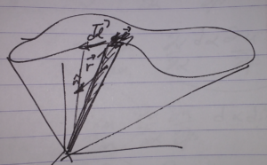
Having proven that the area-integral for a given boundary is independent of the surface that it is evaluated on, the result follows by illustration as hinted in the full problem description. Draw a “cone”, tracing a vector \( \Bx’ \) from the origin to the position line element, and divide that cone up into infinitesimal slices as sketched in fig. 1.

conevectorareafig1

Fig 1. Cone subtended by loop

The area of each of these triangular slices is

\begin{equation}\label{eqn:vectorAreaGriffiths:160}
\inv{2} \Bx’ \cross d\Bl’.
\end{equation}

Summing those triangles proves the result.

(e)

As hinted in the problem, this follows from

\begin{equation}\label{eqn:vectorAreaGriffiths:180}
\int \spacegrad T \cross d\Ba = -\oint T d\Bl.
\end{equation}

Set \( T = \Bc \cdot \Br \), for which

\begin{equation}\label{eqn:vectorAreaGriffiths:240}
\begin{aligned}
\spacegrad T
&= \Be_k \partial_k c_m x_m \\
&= \Be_k c_m \delta_{km} \\
&= \Be_k c_k \\
&= \Bc,
\end{aligned}
\end{equation}

so
\begin{equation}\label{eqn:vectorAreaGriffiths:200}
\begin{aligned}
(\spacegrad T) \cross d\Ba
&=
\int \Bc \cross d\Ba \\
&=
\Bc \cross \int d\Ba \\
&=
\Bc \cross \Ba.
\end{aligned}
\end{equation}

so
\begin{equation}\label{eqn:vectorAreaGriffiths:220}
\Bc \cross \Ba = -\oint (\Bc \cdot \Br) d\Bl,
\end{equation}

or
\begin{equation}\label{eqn:vectorAreaGriffiths:260}
\oint (\Bc \cdot \Br) d\Bl
=
\Ba \cross \Bc.
\end{equation}

References

[1] David Jeffrey Griffiths and Reed College. Introduction to electrodynamics. Prentice hall Upper Saddle River, NJ, 3rd edition, 1999.

Final notes for ECE1254, Modelling of Multiphysics Systems

December 27, 2014 ece1254 , , , , , , , , , , , , , , , , , , , , , , , , , , , , , , , , , , , , , , , , , , , , , , , , , , , , , , , , , , , , , , , , , , , , ,

Capture

I’ve now finished my first grad course, Modelling of Multiphysics Systems, taught by Prof Piero Triverio.

I’ve posted notes for lectures and other material as I was taking the course, but now have an aggregated set of notes for the whole course posted.
This is now updated with all my notes from the lectures, solved problems, additional notes on auxillary topics I wanted to explore (like SVD), plus the notes from the Harmonic Balance report that Mike and I will be presenting in January.

This version of my notes also includes all the matlab figures regenerating using http://www.mathworks.com/matlabcentral/fileexchange/23629-export-fig, which allows a save-as pdf, which rescales much better than Matlab saveas() png’s when embedded in latex.  I’m not sure if that’s the best way to include Matlab figures in latex, but they are at least not fuzzy looking now.

All in all, I’m pretty pleased with my notes for this course.  They are a lot more readable than any of the ones I’ve done for the physics undergrad courses I was taking (https://peeterjoot.com/writing/).  While there was quite a lot covered in this course, the material really only requires an introductory circuits course and some basic math (linear algebra and intro calculus), so is pretty accessible.

This was a fun course.  I recall, back in ancient times when I was a first year student, being unsatisfied with all the ad-hoc strategies we used to solve circuits problems.  This finally answers the questions of how to tackle things more systematically.

Here’s the contents outline for these notes:

Preface
Lecture notes
1 nodal analysis
1.1 In slides
1.2 Mechanical structures example
1.3 Assembling system equations automatically. Node/branch method
1.4 Nodal Analysis
1.5 Modified nodal analysis (MNA)
2 solving large systems
2.1 Gaussian elimination
2.2 LU decomposition
2.3 Problems
3 numerical errors and conditioning
3.1 Strict diagonal dominance
3.2 Exploring uniqueness and existence
3.3 Perturbation and norms
3.4 Matrix norm
4 singular value decomposition, and conditioning number
4.1 Singular value decomposition
4.2 Conditioning number
5 sparse factorization
5.1 Fill ins
5.2 Markowitz product
5.3 Markowitz reordering
5.4 Graph representation
6 gradient methods
6.1 Summary of factorization costs
6.2 Iterative methods
6.3 Gradient method
6.4 Recap: Summary of Gradient method
6.5 Conjugate gradient method
6.6 Full Algorithm
6.7 Order analysis
6.8 Conjugate gradient convergence
6.9 Gershgorin circle theorem
6.10 Preconditioning
6.11 Symmetric preconditioning
6.12 Preconditioned conjugate gradient
6.13 Problems
7 solution of nonlinear systems
7.1 Nonlinear systems
7.2 Richardson and Linear Convergence
7.3 Newton’s method
7.4 Solution of N nonlinear equations in N unknowns
7.5 Multivariable Newton’s iteration
7.6 Automatic assembly of equations for nonlinear system
7.7 Damped Newton’s method
7.8 Continuation parameters
7.9 Singular Jacobians
7.10 Struts and Joints, Node branch formulation
7.11 Problems
8 time dependent systems
8.1 Assembling equations automatically for dynamical systems
8.2 Numerical solution of differential equations
8.3 Forward Euler method
8.4 Backward Euler method
8.5 Trapezoidal rule (TR)
8.6 Nonlinear differential equations
8.7 Analysis, accuracy and stability (Dt ! 0)
8.8 Residual for LMS methods
8.9 Global error estimate
8.10 Stability
8.11 Stability (continued)
8.12 Problems
9 model order reduction
9.1 Model order reduction
9.2 Moment matching
9.3 Model order reduction (cont).
9.4 Moment matching
9.5 Truncated Balanced Realization (1000 ft overview)
9.6 Problems
Final report
10 harmonic balance
10.1 Abstract
10.2 Introduction
10.2.1 Modifications to the netlist syntax
10.3 Background
10.3.1 Discrete Fourier Transform
10.3.2 Harmonic Balance equations
10.3.3 Frequency domain representation of MNA equations
10.3.4 Example. RC circuit with a diode.
10.3.5 Jacobian
10.3.6 Newton’s method solution
10.3.7 Alternative handling of the non-linear currents and Jacobians
10.4 Results
10.4.1 Low pass filter
10.4.2 Half wave rectifier
10.4.3 AC to DC conversion
10.4.4 Bridge rectifier
10.4.5 Cpu time and error vs N
10.4.6 Taylor series non-linearities
10.4.7 Stiff systems
10.5 Conclusion
10.6 Appendices
10.6.1 Discrete Fourier Transform inversion
Appendices
a singular value decomposition
b basic theorems and definitions
c norton equivalents
d stability of discretized linear differential equations
e laplace transform refresher
f discrete fourier transform
g harmonic balance, rough notes
g.1 Block matrix form, with physical parameter ordering
g.2 Block matrix form, with frequency ordering
g.3 Representing the linear sources
g.4 Representing non-linear sources
g.5 Newton’s method
g.6 A matrix formulation of Harmonic Balance non-linear currents
h matlab notebooks
i mathematica notebooks
Index
Bibliography

A matrix formulation of the Harmonic Balance method non-linear currents

December 14, 2014 ece1254 , , , , , ,

[Click here for a PDF of this post with nicer formatting]

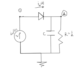
Because it was simple, a coordinate expansion of the Jacobian of the non-linear currents was good to get a feeling for the structure of the equations. However, a Jacobian of that form is impossibly slow to compute for larger \( N \). It seems plausible that eliminating the coordinate expansion, expressing both the currrent and the Jacobian directly in terms of the Harmonic Balance unknowns vector \( \BV \), would lead to a simpler set of equations that could be implemented in a computationally more effective way. To aid in this discovery, consider the simple RC load diode circuit of fig. 1. It’s not too hard to start from scratch with the time domain nodal equations for this circuit, which are

diodeWithResistorAndCapacitorFig1

fig. 1. Simple diode and resistor circuit


  1. \( 0 = i_s – i_d \)
  2. \( Z v^{(2)} + C dv^{(2)}/dt = i_d \)
  3. \( i_d = I_0 \lr{ e^{(v^{(1)} – v^{(2)})/V_T} – 1} \)

To setup for matrix form, let

\begin{equation}\label{eqn:diodeRLCSample:1240}
\Bv(t) =
\begin{bmatrix}
v^{(1)}(t) \\
v^{(2)}(t) \\
\end{bmatrix}
\end{equation}
\begin{equation}\label{eqn:diodeRLCSample:1140}
\BG =
\begin{bmatrix}
0 & 0 \\
0 & Z \\
\end{bmatrix}
\end{equation}
\begin{equation}\label{eqn:diodeRLCSample:1160}
\BC =
\begin{bmatrix}
0 & 0 \\
0 & C \\
\end{bmatrix}
\end{equation}
\begin{equation}\label{eqn:diodeRLCSample:1180}
\Bd =
\begin{bmatrix}
1 \\
-1
\end{bmatrix}
\end{equation}
\begin{equation}\label{eqn:diodeRLCSample:1200}
\Bb =
\begin{bmatrix}
1 \\
0
\end{bmatrix},
\end{equation}

so that the time domain equations can be written as

\begin{equation}\label{eqn:diodeRLCSample:1220}
\BG \Bv(t)
+ \BC \Bv'(t)
=
\Bb i_s(t)
+
I_0
\Bd
\lr{
e^{ (v^{(1)}(t) – v^{(2)}(t))/V_T} – 1
}
=
\begin{bmatrix}
\Bb & -I_0 \Bd
\end{bmatrix}
\begin{bmatrix}
i_s(t) \\
1
\end{bmatrix}
+
I_0 \Bd
e^{ (v^{(1)}(t) – v^{(2)}(t))/V_T}.
\end{equation}

Harmonic Balance is essentially the assumption that the input and outputs are assumed to be a bandwidth limited periodic signal, and the non-linear components can be approximated by the same

\begin{equation}\label{eqn:diodeRLCSample:1260}
i_s(t) = \sum_{n=-N}^N I^{(s)}_n e^{ j \omega_0 n t },
\end{equation}
\begin{equation}\label{eqn:diodeRLCSample:1280}
v^{(k)}(t) =
\sum_{n=-N}^N V^{(k)}_n e^{ j \omega_0 n t },
\end{equation}
\begin{equation}\label{eqn:diodeRLCSample:1300}
\epsilon(t) =
e^{ (v^{(1)}(t) – v^{(2)}(t))/V_T}
\simeq
\sum_{n=-N}^N E_n e^{ j \omega_0 n t },
\end{equation}

The approximation in \ref{eqn:diodeRLCSample:1300} is an equality only at the Nykvist sampling times \( t_k = T k/(2 N + 1) \). The Fourier series provides a periodic extension to other times that will approximate the underlying periodic non-linear relation.

With all the time dependence locked into the exponentials, the derivatives are really easy to calculate

\begin{equation}\label{eqn:diodeRLCSample:1281}
\frac{d}{dt} v^{(k)}(t) =
\sum_{n=-N}^N j \omega_0 n V^{(k)}_n e^{ j \omega_0 n t }.
\end{equation}

Inserting all of these into \ref{eqn:diodeRLCSample:1220} gives

\begin{equation}\label{eqn:diodeRLCSample:1320}
\sum_{n=-N}^N e^{ j \omega_0 n t} \lr{ \BG + j \omega_0 n \BC }
\begin{bmatrix}
V^{(1)}_n \\
V^{(2)}_n \\
\end{bmatrix}
=
\sum_{n=-N}^N e^{ j \omega_0 n t}
\lr{
-I_0 \Bd \delta_{n 0}
+
\Bb I^{(s)}_n
+ I_0 \Bd E_n
}.
\end{equation}

The periodic assumption requires equality for each \( e^{j \omega_0 n t} \), or

\begin{equation}\label{eqn:diodeRLCSample:1340}
\lr{ \BG + j \omega_0 n \BC }
\begin{bmatrix}
V^{(1)}_n \\
V^{(2)}_n \\
\end{bmatrix}
=
-I_0 \Bd \delta_{n 0}
+
\Bb I^{(s)}_n
+ I_0 \Bd E_n.
\end{equation}

For illustration, consider the \( N = 1 \) case, where the block matrix form is

\begin{equation}\label{eqn:diodeRLCSample:1360}
\begin{bmatrix}
\BG + j \omega_0 (-1) \BC & 0 & 0 \\
0 & \BG + j \omega_0 (0) \BC & 0 \\
0 & 0 & \BG + j \omega_0 (1) \BC
\end{bmatrix}
\begin{bmatrix}
\begin{bmatrix}
V^{(1)}_{-1} \\
V^{(2)}_{-1} \\
\end{bmatrix} \\
\begin{bmatrix}
V^{(1)}_{0} \\
V^{(2)}_{0} \\
\end{bmatrix} \\
\begin{bmatrix}
V^{(1)}_{1} \\
V^{(2)}_{1} \\
\end{bmatrix}
\end{bmatrix}
=
\begin{bmatrix}
\Bb I^{(s)}_{-1} \\
\Bb I^{(s)}_{0} – I_0 \Bd \\
\Bb I^{(s)}_{1} \\
\end{bmatrix}
+
I_0
\begin{bmatrix}
\Bd E_{-1} \\
\Bd E_{0} \\
\Bd E_{1} \\
\end{bmatrix}.
\end{equation}

The structure of this equation is

\begin{equation}\label{eqn:diodeRLCSample:1380}
\BY \BV = \BI + \mathcal{I}(\BV),
\end{equation}

The non-linear current \( \mathcal{I}(\BV) \) needs to be examined further. How much of this can be precomputed, and what is the simplest way to compute the Jacobian? With

\begin{equation}\label{eqn:diodeRLCSample:1400}
\BE =
\begin{bmatrix}
E_{-1} \\
E_{0} \\
E_{1} \\
\end{bmatrix}, \qquad
\Bepsilon =
\begin{bmatrix}
\epsilon_{-1} \\
\epsilon_{0} \\
\epsilon_{1} \\
\end{bmatrix},
\end{equation}

the non-linear current is

\begin{equation}\label{eqn:diodeRLCSample:1420}
\mathcal{I} =
I_0
\begin{bmatrix}
\Bd E_{-1} \\
\Bd E_{0} \\
\Bd E_{1} \\
\end{bmatrix}
=
I_0
\begin{bmatrix}
\Bd \begin{bmatrix} 1 & 0 & 0 \end{bmatrix} \BE \\
\Bd \begin{bmatrix} 0 & 1 & 0 \end{bmatrix} \BE \\
\Bd \begin{bmatrix} 0 & 0 & 1 \end{bmatrix} \BE
\end{bmatrix}
=
I_0
\begin{bmatrix}
\Bd & 0 & 0 \\
0 & \Bd & 0 \\
0 & 0 & \Bd
\end{bmatrix}
\BF^{-1} \Bepsilon
\end{equation}

In the last step \( \BE = \BF^{-1} \Bepsilon \) has been factored out (in its inverse Fourier form). With

\begin{equation}\label{eqn:diodeRLCSample:1480}
\BD =
\begin{bmatrix}
\Bd & 0 & 0 \\
0 & \Bd & 0 \\
0 & 0 & \Bd \\
\end{bmatrix},
\end{equation}

the current is

\begin{equation}\label{eqn:diodeRLCSample:1540}
\boxed{
\mathcal{I}(\BV) =
I_0 \BD \BF^{-1} \Bepsilon(\BV).
}
\end{equation}

The next step is finding an appropriate form for \( \Bepsilon \)

\begin{equation}\label{eqn:diodeRLCSample:1440}
\begin{aligned}
\Bepsilon &=
\begin{bmatrix}
\epsilon(t_{-1}) \\
\epsilon(t_{0}) \\
\epsilon(t_{1}) \\
\end{bmatrix} \\
&=
\begin{bmatrix}
\exp\lr{ \lr{ v^{(1)}_{-1} – v^{(2)}_{-1} }/V_T } \\
\exp\lr{ \lr{ v^{(1)}_{0} – v^{(2)}_{0} }/V_T } \\
\exp\lr{ \lr{ v^{(1)}_{1} – v^{(2)}_{1} }/V_T }
\end{bmatrix} \\
&=
\begin{bmatrix}
\exp\lr{
\begin{bmatrix}
1 & 0 & 0
\end{bmatrix}
\lr{ \Bv^{(1)} – \Bv^{(2)} }/V_T } \\
\exp\lr{
\begin{bmatrix}
0 & 1 & 0
\end{bmatrix}
\lr{ \Bv^{(1)} – \Bv^{(2)} }/V_T } \\
\exp\lr{
\begin{bmatrix}
0 & 0 & 1
\end{bmatrix}
\lr{ \Bv^{(1)} – \Bv^{(2)} }/V_T } \\
\end{bmatrix} \\
&=
\begin{bmatrix}
\exp\lr{
\begin{bmatrix}
1 & 0 & 0
\end{bmatrix}
\BF
\lr{ \BV^{(1)} – \BV^{(2)} }/V_T } \\
\exp\lr{
\begin{bmatrix}
0 & 1 & 0
\end{bmatrix}
\BF
\lr{ \BV^{(1)} – \BV^{(2)} }/V_T } \\
\exp\lr{
\begin{bmatrix}
0 & 0 & 1
\end{bmatrix}
\BF
\lr{ \BV^{(1)} – \BV^{(2)} }/V_T } \\
\end{bmatrix}.
\end{aligned}
\end{equation}

It would be nice to have the difference of frequency domain vectors expressed in terms of \( \BV \), which can be done with a bit of rearrangement

\begin{equation}\label{eqn:diodeRLCSample:1460}
\begin{aligned}
\BV^{(1)} – \BV^{(2)}
&=
\begin{bmatrix}
V^{(1)}_{-1} – V^{(2)}_{-1} \\
V^{(1)}_{0} – V^{(2)}_{0} \\
V^{(1)}_{1} – V^{(2)}_{1} \\
\end{bmatrix} \\
&=
\begin{bmatrix}
1 & -1 & 0 & 0 & 0 & 0 \\
0 & 0 & 1 & -1 & 0 & 0 \\
0 & 0 & 0 & 0 & 1 & -1 \\
\end{bmatrix}
\begin{bmatrix}
V_{-1}^{(1)} \\
V_{-1}^{(2)} \\
V_{0}^{(1)} \\
V_{0}^{(2)} \\
V_{1}^{(1)} \\
V_{1}^{(2)} \\
\end{bmatrix} \\
&=
\begin{bmatrix}
\Bd^\T & 0 & 0 \\
0 & \Bd^\T & 0 \\
0 & 0 & \Bd^\T \\
\end{bmatrix}
\BV \\
&= \BD^\T \BV,
\end{aligned}
\end{equation}

\begin{equation}\label{eqn:diodeRLCSample:1520}
\BH
=
\BF \BD^\T /V_T
=
\begin{bmatrix}
\Bh_1^\T \\
\Bh_2^\T \\
\Bh_3^\T
\end{bmatrix},
\end{equation}

which allows the non-linear current to can now be completely expressed in terms of \( \BV \).

\begin{equation}\label{eqn:diodeRLCSample:1560}
\boxed{
\Bepsilon(\BV)
=
\begin{bmatrix}
e^{\Bh_1^\T \BV} \\
e^{\Bh_2^\T \BV} \\
e^{\Bh_3^\T \BV} \\
\end{bmatrix}.
}
\end{equation}

Jacobian

With a compact matrix representation of the non-linear current, attention can now be turned to the Jacobian of the non-linear current. Let \( \BA = I_0 \BD \BF^{-1} = [ a_{ij} ]_{ij} \), the current (with summation implied) is

\begin{equation}\label{eqn:diodeRLCSample:1580}
\mathcal{I} =
\begin{bmatrix}
a_{ik} \epsilon_k,
\end{bmatrix}
\end{equation}

with coordinates

\begin{equation}\label{eqn:diodeRLCSample:1600}
\mathcal{I}_i = a_{ik} \epsilon_k = a_{ik} \exp\lr{ \Bh_k^\T \BV }.
\end{equation}

so the Jacobian components are

\begin{equation}\label{eqn:diodeRLCSample:1620}
[\BJ^{\mathcal{I}}]_{ij}
=
a_{ik} \epsilon_k = a_{ik}
\PD{V_j}{}
\exp\lr{ \Bh_k^\T \BV }
=
a_{ik}
h_{kj}
\exp\lr{ \Bh_k^\T \BV }.
\end{equation}

Factoring out \( \BU = [h_{ij} \exp\lr{ \Bh_i^\T \BV }]_{ij} \),

\begin{equation}\label{eqn:diodeRLCSample:1640}
\BJ^{\mathcal{I}}
= \BA \BU
=
\BA
\begin{bmatrix}
\begin{bmatrix} h_{11} & h_{12} & \cdots h_{1, R(2 N + 1)}\end{bmatrix} \exp\lr{ \Bh_1^\T \BV } \\
\begin{bmatrix} h_{21} & h_{22} & \cdots h_{2, R(2 N + 1)}\end{bmatrix} \exp\lr{ \Bh_2^\T \BV } \\
\begin{bmatrix} h_{31} & h_{32} & \cdots h_{3, R(2 N + 1)}\end{bmatrix} \exp\lr{ \Bh_3^\T \BV } \\
\end{bmatrix}
=
\BA
\begin{bmatrix}
\Bh_1^\T \exp\lr{ \Bh_1^\T \BV } \\
\Bh_2^\T \exp\lr{ \Bh_2^\T \BV } \\
\Bh_3^\T \exp\lr{ \Bh_3^\T \BV } \\
\end{bmatrix}.
\end{equation}

A quick sanity check of dimensions seems worthwhile, and shows that all is well

  • \( \BA \) : \( R(2 N + 1) \times 2 N + 1 \)
  • \( \BU \) : \( 2 N + 1 \times R(2 N + 1) \)
  • \( \BJ^{\mathcal{I}} \) : \( R(2 N + 1) \times R(2 N + 1) \)

The Jacobian of the non-linear current is now completely determined

\begin{equation}\label{eqn:diodeRLCSample:1660}
\boxed{
\BJ^{\mathcal{I}}( \BV ) =
I_0 \BD \BF^{-1}
\begin{bmatrix}
\Bh_1^\T \exp\lr{ \Bh_1^\T \BV } \\
\Bh_2^\T \exp\lr{ \Bh_2^\T \BV } \\
\Bh_3^\T \exp\lr{ \Bh_3^\T \BV } \\
\end{bmatrix}.
}
\end{equation}

Newton’s method solution

All the pieces required for a Newton’s method solution are now in place. The goal is to find a value of \( \BV \) that provides the zero

\begin{equation}\label{eqn:diodeRLCSample:1680}
f(\BV) = \BY \BV – \BI – \mathcal{I}(\BV).
\end{equation}

Expansion to first order around an initial guess \( \BV^0 \), gives

\begin{equation}\label{eqn:diodeRLCSample:1700}
f( \BV^0 + \Delta \BV ) = f(\BV^0) + \BJ(\BV^0) \Delta \BV \approx 0,
\end{equation}

where the full Jacobian of \( f(\BV) \) is

\begin{equation}\label{eqn:diodeRLCSample:1720}
\BJ(\BV) = \BY – \BJ^{\mathcal{I}}(\BV).
\end{equation}

The Newton’s method refinement of the initial guess follows by inversion

\begin{equation}\label{eqn:diodeRLCSample:1740}
\Delta \BV = -\lr{ \BY – \BJ^{\mathcal{I}}(\BV^0) }^{-1} f(\BV^0).
\end{equation}