math and physics play

Fresnel angular sum and difference formulas

November 22, 2016 math and physics play , ,

[Click here for a PDF of this post with nicer formatting]

In [1] are some sum and angle difference formulations for the Fresnel formulas given a \( \mu_1 = \mu_2 \) constraint. The proof of these trig Fresnel equations is left to an exercise, and will be derived here.

We need a couple trig identities to start with.

\begin{equation}\label{eqn:fresnelSumAndDifferenceAngleFormulas:20}
\begin{aligned}
\sin(a + b)
&=
\textrm{Im}\lr{ e^{j(a + b)} } \\
&=
\textrm{Im}\lr{
e^{ja} e^{+ jb}
} \\
&=
\textrm{Im}\lr{
(\cos a + j \sin a) (\cos b + j \sin b)
} \\
&=
\sin a \cos b + \cos a \sin b.
\end{aligned}
\end{equation}

Allowing for both signs we have

\begin{equation}\label{eqn:fresnelSumAndDifferenceAngleFormulas:240}
\begin{aligned}
\sin(a + b) &= \sin a \cos b + \cos a \sin b \\
\sin(a – b) &= \sin a \cos b – \cos a \sin b.
\end{aligned}
\end{equation}

The mixed sine and cosine product can be expressed as a sum of sines

\begin{equation}\label{eqn:fresnelSumAndDifferenceAngleFormulas:40}
2 \sin a \cos b = \sin(a + b) + \sin(a – b).
\end{equation}

With \( 2 x = a + b, 2 y = a – b \), or \( a = x + y, b = x – y \), we find

\begin{equation}\label{eqn:fresnelSumAndDifferenceAngleFormulas:60}
\begin{aligned}
2 \sin(x + y) \cos (x – y) &= \sin( 2 x ) + \sin( 2 y ) \\
2 \sin(x – y) \cos (x + y) &= \sin( 2 x ) – \sin( 2 y ).
\end{aligned}
\end{equation}

Returning to the problem. When \( \mu_1 = \mu_2 \) the Fresnel equations were found to be

\begin{equation}\label{eqn:fresnelSumAndDifferenceAngleFormulas:100}
\begin{aligned}
r^{\textrm{TE}} &= \frac { n_1 \cos\theta_i – n_2 \cos\theta_t } { n_1 \cos\theta_i + n_2 \cos\theta_t } \\
r^{\textrm{TM}} &= \frac{n_2 \cos\theta_i – n_1 \cos\theta_t }{ n_2 \cos\theta_i + n_1 \cos\theta_t } \\
t^{\textrm{TE}} &= \frac{ 2 n_1 \cos\theta_i } { n_1 \cos\theta_i + n_2 \cos\theta_t } \\
t^{\textrm{TM}} &= \frac{2 n_1 \cos\theta_i }{ n_2 \cos\theta_i + n_1 \cos\theta_t }.
\end{aligned}
\end{equation}

Using Snell’s law, one of \( n_1, n_2 \) can be eliminated, for example

\begin{equation}\label{eqn:fresnelSumAndDifferenceAngleFormulas:120}
n_1 = n_2 \frac{\sin \theta_t}{\sin\theta_i}.
\end{equation}

Inserting this and proceeding with the application of the trig identities above, we have

\begin{equation}\label{eqn:fresnelSumAndDifferenceAngleFormulas:160}
\begin{aligned}
r^{\textrm{TE}}
&= \frac { n_2 \frac{\sin\theta_t}{\sin\theta_i} \cos\theta_i – n_2 \cos\theta_t } { n_2 \frac{\sin\theta_t}{\sin\theta_i} \cos\theta_i + n_2 \cos\theta_t } \\
&=
\frac {
\sin\theta_t \cos\theta_i – \cos\theta_t \sin\theta_i
} {
\sin\theta_t \cos\theta_i + \cos\theta_t \sin\theta_i
} \\
&=
\frac {
\sin( \theta_t – \theta_i )
} {
\sin( \theta_t + \theta_i )
}
\end{aligned}
\end{equation}
\begin{equation}\label{eqn:fresnelSumAndDifferenceAngleFormulas:180}
\begin{aligned}
r^{\textrm{TM}}
&= \frac{n_2 \cos\theta_i – n_2 \frac{\sin\theta_t}{\sin\theta_i} \cos\theta_t }{ n_2 \cos\theta_i + n_2 \frac{\sin\theta_t}{\sin\theta_i} \cos\theta_t } \\
&= \frac{
\sin\theta_i \cos\theta_i – \sin\theta_t \cos\theta_t
}{
\sin\theta_i \cos\theta_i + \sin\theta_t \cos\theta_t
} \\
&= \frac{\inv{2} \sin(2 \theta_i) – \inv{2} \sin(2 \theta_t) }{ \inv{2} \sin(2 \theta_i) + \inv{2} \sin(2 \theta_t) } \\
&= \frac
{\sin(\theta_i – \theta_t)\cos(\theta_i + \theta_t) }
{\sin(\theta_i + \theta_t)\cos(\theta_i – \theta_t) } \\
&=
\frac
{\tan(\theta_i -\theta_t)}
{\tan(\theta_i +\theta_t)}
\end{aligned}
\end{equation}
\begin{equation}\label{eqn:fresnelSumAndDifferenceAngleFormulas:200}
\begin{aligned}
t^{\textrm{TE}}
&= \frac{ 2 n_2 \frac{\sin\theta_t}{\sin\theta_i} \cos\theta_i } { n_2 \frac{\sin\theta_t}{\sin\theta_i} \cos\theta_i + n_2 \cos\theta_t } \\
&= \frac{ 2 \sin\theta_t \cos\theta_i } { \sin\theta_t \cos\theta_i + \cos\theta_t \sin\theta_i } \\
&= \frac{ 2 \sin\theta_t \cos\theta_i }
{ \sin(\theta_i + \theta_t) }
\end{aligned}
\end{equation}
\begin{equation}\label{eqn:fresnelSumAndDifferenceAngleFormulas:220}
\begin{aligned}
t^{\textrm{TM}}
&= \frac{2 n_2 \frac{\sin\theta_t}{\sin\theta_i} \cos\theta_i }{ n_2 \cos\theta_i + n_2 \frac{\sin\theta_t}{\sin\theta_i} \cos\theta_t } \\
&= \frac{2 \sin\theta_t \cos\theta_i }{ \sin\theta_i \cos\theta_i + \sin\theta_t \cos\theta_t } \\
&= \frac{2 \sin\theta_t \cos\theta_i }
{ \inv{2} \sin(2 \theta_i) + \inv{2} \sin(2 \theta_t) } \\
&= \frac{2 \sin\theta_t \cos\theta_i }
{ \sin(\theta_i + \theta_t) \cos(\theta_i – \theta_t) }
\end{aligned}
\end{equation}

References

[1] E. Hecht. Optics. 1998.

Normal transmission and reflection through two interfaces

November 21, 2016 math and physics play , , , ,

[Click here for a PDF of this post with nicer formatting]

Motivation

In class an outline of normal transmission through a slab was presented. Let’s go through the details.

Normal incidence

The geometry of a two interface configuration is sketched in fig. 1.


l10twointerfacesfig1

fig. 1. Two interface transmission.

Given a normal incident ray with magnitude \( A \), the respective forward and backwards rays in each the mediums can be written as

    [I]

  1. \begin{equation}\label{eqn:twoInterfaceNormal:20}
    \begin{aligned}
    A e^{-j k_1 z} \\
    A r e^{j k_1 z} \\
    \end{aligned}
    \end{equation}
  2. \begin{equation}\label{eqn:twoInterfaceNormal:40}
    C e^{-j k_2 z} \\
    D e^{j k_2 z} \\
    \end{equation}
  3. \begin{equation}\label{eqn:twoInterfaceNormal:60}
    A t e^{-j k_3 (z-d)}
    \end{equation}

Matching at \( z = 0 \) gives
\begin{equation}\label{eqn:twoInterfaceNormal:80}
\begin{aligned}
A t_{12} + r_{21} D &= C \\
A r &= A r_{12} + D t_{21},
\end{aligned}
\end{equation}

whereas matching at \( z = d \) gives

\begin{equation}\label{eqn:twoInterfaceNormal:100}
\begin{aligned}
A t &= C e^{-j k_2 d} t_{23} \\
D e^{j k_2 d} &= C e^{-j k_2 d} r_{23}
\end{aligned}
\end{equation}

We have four linear equations in four unknowns \( r, t, C, D \), but only care about solving for \( r, t \). Let’s write \(
\gamma = e^{ j k_2 d }, C’ = C/A, D’ = D/A \), for

\begin{equation}\label{eqn:twoInterfaceNormal:120}
\begin{aligned}
t_{12} + r_{21} D’ &= C’ \\
r &= r_{12} + D’ t_{21} \\
t \gamma &= C’ t_{23} \\
D’ \gamma^2 &= C’ r_{23}
\end{aligned}
\end{equation}

Solving for \( C’, D’ \) we get

\begin{equation}\label{eqn:twoInterfaceNormal:140}
\begin{aligned}
D’ \lr{ \gamma^2 – r_{21} r_{23} } &= t_{12} r_{23} \\
C’ \lr{ \gamma^2 – r_{21} r_{23} } &= t_{12} \gamma^2,
\end{aligned}
\end{equation}

so

\begin{equation}\label{eqn:twoInterfaceNormal:160}
\begin{aligned}
r &= r_{12} + \frac{t_{12} t_{21} r_{23} }{\gamma^2 – r_{21} r_{23} } \\
t &= t_{23} \frac{ t_{12} \gamma }{\gamma^2 – r_{21} r_{23} }.
\end{aligned}
\end{equation}

With \( \phi = -j k_2 d \), or \( \gamma = e^{-j\phi} \), we have

\begin{equation}\label{eqn:twoInterfaceNormal:180}
\boxed{
\begin{aligned}
r &= r_{12} + \frac{t_{12} t_{21} r_{23} e^{2 j \phi} }{1 – r_{21} r_{23} e^{2 j \phi}} \\
t &= \frac{ t_{12} t_{23} e^{j\phi}}{1 – r_{21} r_{23} e^{2 j \phi}}.
\end{aligned}
}
\end{equation}

A slab

When the materials in region I, and III are equal, then \( r_{12} = r_{32} \). For a TE mode, we have

\begin{equation}\label{eqn:twoInterfaceNormal:200}
r_{12}
=
\frac{\mu_2 k_{1z} – \mu_1 k_{2z}}{\mu_2 k_{1z} + \mu_1 k_{2z}}
= -r_{21}.
\end{equation}

so the reflection and transmission coefficients are

\begin{equation}\label{eqn:twoInterfaceNormal:220}
\begin{aligned}
r^{\textrm{TE}} &= r_{12} \lr{ 1 – \frac{t_{12} t_{21} e^{2 j \phi} }{1 – r_{21}^2 e^{2 j \phi}} } \\
t^{\textrm{TE}} &= \frac{ t_{12} t_{21} e^{j\phi}}{1 – r_{21}^2 e^{2 j \phi}}.
\end{aligned}
\end{equation}

It’s possible to produce a matched condition for which \( r_{12} = r_{21} = 0 \), by selecting

\begin{equation}\label{eqn:twoInterfaceNormal:240}
\begin{aligned}
0
&= \mu_2 k_{1z} – \mu_1 k_{2z} \\
&= \mu_1 \mu_2 \lr{ \inv{\mu_1} k_{1z} – \inv{\mu_2} k_{2z} } \\
&= \mu_1 \mu_2 \omega \lr{ \frac{1}{v_1 \mu_1} \theta_1 – \frac{1}{v_2 \mu_2} \theta_2 },
\end{aligned}
\end{equation}

or

\begin{equation}\label{eqn:twoInterfaceNormal:260}
\inv{\eta_1} \cos\theta_1 = \inv{\eta_2} \cos\theta_2,
\end{equation}

so the matching condition for normal incidence is just

\begin{equation}\label{eqn:twoInterfaceNormal:280}
\eta_1 = \eta_2.
\end{equation}

Given this matched condition, the transmission coefficient for the 1,2 interface is

\begin{equation}\label{eqn:twoInterfaceNormal:300}
\begin{aligned}
t_{12}
&= \frac{2 \mu_2 k_{1z}}{\mu_2 k_{1z} + \mu_1 k_{2z}} \\
&= \frac{2 \mu_2 k_{1z}}{2 \mu_2 k_{1z} } \\
&= 1,
\end{aligned}
\end{equation}

so the matching condition yields
\begin{equation}\label{eqn:twoInterfaceNormal:320}
\begin{aligned}
t
&=
t_{12} t_{21} e^{j\phi} \\
&=
e^{j\phi} \\
&=
e^{-j k_2 d}.
\end{aligned}
\end{equation}

Normal transmission through a matched slab only introduces a phase delay.

ECE1228H Electromagnetic Theory. Lecture 10: Fresnel relations. Taught by Prof. M. Mojahedi

November 20, 2016 math and physics play , , , ,

[Click here for a PDF of this post with nicer formatting]

Motivation

In class, an overview of the Fresnel relations for a TE mode electric field were presented. Here’s a fleshing out of the details is presented, as well as the equivalent for the TM mode.

Single interface TE mode.

The Fresnel reflection geometry for an electric field \( \BE \) parallel to the interface (TE mode) is sketched in fig. 1.

fresneltefig1

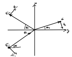
fig. 1. Electric field TE mode Fresnel geometry.

\begin{equation}\label{eqn:emtLecture10:20}
\boldsymbol{\mathcal{E}}_i = \Be_2 E_i e^{j \omega t – j \Bk_{i} \cdot \Bx },
\end{equation}

with an assumption that this field maintains it’s polarization in both its reflected and transmitted components, so that

\begin{equation}\label{eqn:emtLecture10:40}
\boldsymbol{\mathcal{E}}_r = \Be_2 r E_i e^{j \omega t – j \Bk_{r} \cdot \Bx },
\end{equation}

and
\begin{equation}\label{eqn:emtLecture10:60}
\boldsymbol{\mathcal{E}}_t = \Be_2 t E_i e^{j \omega t – j \Bk_{t} \cdot \Bx },
\end{equation}

Measuring the angles \( \theta_i, \theta_r, \theta_t \) from the normal, with \( i = \Be_3 \Be_1 \) the wave vectors are

\begin{equation}\label{eqn:emtLecture10:620}
\begin{aligned}
\Bk_{i} &= \Be_3 k_1 e^{i\theta_i} = k_1\lr{ \Be_3 \cos\theta_i + \Be_1\sin\theta_i } \\
\Bk_{r} &= -\Be_3 k_1 e^{-i\theta_r} = k_1 \lr{ -\Be_3 \cos\theta_r + \Be_1 \sin\theta_r } \\
\Bk_{t} &= \Be_3 k_2 e^{i\theta_t} = k_2 \lr{ \Be_3 \cos\theta_t + \Be_1 \sin\theta_t }
\end{aligned}
\end{equation}

So the time harmonic electric fields are

\begin{equation}\label{eqn:emtLecture10:640}
\begin{aligned}
\BE_i &= \Be_2 E_i \exp\lr{ – j k_1 \lr{ z\cos\theta_i + x \sin\theta_i} } \\
\BE_r &= \Be_2 r E_i \exp\lr{ – j k_1 \lr{ -z \cos\theta_r + x \sin\theta_r}} \\
\BE_t &= \Be_2 t E_i \exp\lr{ – j k_2 \lr{ z \cos\theta_t + x \sin\theta_t}}.
\end{aligned}
\end{equation}

The magnetic fields follow from Faraday’s law

\begin{equation}\label{eqn:emtLecture10:900}
\begin{aligned}
\BH
&= \inv{-j \omega \mu } \spacegrad \cross \BE \\
&= \inv{-j \omega \mu } \spacegrad \cross \Be_2 e^{-j \Bk \cdot \Bx} \\
&= \inv{j \omega \mu } \Be_2 \cross \spacegrad e^{-j \Bk \cdot \Bx} \\
&= -\inv{\omega \mu } \Be_2 \cross \Bk e^{-j \Bk \cdot \Bx} \\
&= \inv{\omega \mu } \Bk \cross \BE
\end{aligned}
\end{equation}

We have

\begin{equation}\label{eqn:emtLecture10:920}
\begin{aligned}
\kcap_{i} \cross \Be_2 &= -\Be_1 \cos\theta_i + \Be_3\sin\theta_i \\
\kcap_{r} \cross \Be_2 &= \Be_1 \cos\theta_r + \Be_3 \sin\theta_r \\
\kcap_{t} \cross \Be_2 &= -\Be_1 \cos\theta_t + \Be_3 \sin\theta_t,
\end{aligned}
\end{equation}

Note that
\begin{equation}\label{eqn:emtLecture10:1500}
\begin{aligned}
\frac{k}{\omega \mu}
&=
\frac{k}{k v \mu} \\
&=
\frac{\sqrt{\mu\epsilon}}{\mu} \\
&=\sqrt
{
\frac{\epsilon}{\mu}
} \\
&=
\inv{\eta}.
\end{aligned}
\end{equation}

so
\begin{equation}\label{eqn:emtLecture10:940}
\begin{aligned}
\BH_{i} &= \frac{ E_i}{\eta_1} \lr{ -\Be_1 \cos\theta_i + \Be_3\sin\theta_i } \exp\lr{ – j k_1 \lr{ z\cos\theta_i + x \sin\theta_i} } \\
\BH_{r} &= \frac{ r E_i}{\eta_1} \lr{ \Be_1 \cos\theta_r + \Be_3 \sin\theta_r } \exp\lr{ – j k_1 \lr{ -z \cos\theta_r + x \sin\theta_r}} \\
\BH_{t} &= \frac{ t E_i}{\eta_2} \lr{ -\Be_1 \cos\theta_t + \Be_3 \sin\theta_t } \exp\lr{ – j k_2 \lr{ z \cos\theta_t + x \sin\theta_t}}.
\end{aligned}
\end{equation}

The boundary conditions at \( z = 0 \) with \( \ncap = \Be_3 \) are

\begin{equation}\label{eqn:emtLecture10:960}
\begin{aligned}
\ncap \cross \BH_1 &= \ncap \cross \BH_2 \\
\ncap \cdot \BB_1 &= \ncap \cdot \BB_2 \\
\ncap \cross \BE_1 &= \ncap \cross \BE_2 \\
\ncap \cdot \BD_1 &= \ncap \cdot \BD_2,
\end{aligned}
\end{equation}

At \( x = 0 \), this is

\begin{equation}\label{eqn:emtLecture10:1060}
\begin{aligned}
-\frac{1}{\eta_1} \cos\theta_i + \frac{r }{\eta_1} \cos\theta_r &= -\frac{t }{\eta_2} \cos\theta_t \\
k_1 \sin\theta_i + k_1 r \sin\theta_r &= k_2 t \sin\theta_t \\
1 + r &= t
\end{aligned}
\end{equation}

When \( t = 0 \) the latter two equations give Shell’s first law

\begin{equation}\label{eqn:emtLecture10:1080}
\boxed{
\sin\theta_i = \sin\theta_r.
}
\end{equation}

Assuming this holds for all \( r, t \) we have

\begin{equation}\label{eqn:emtLecture10:1120}
k_1 \sin\theta_i (1 + r ) = k_2 t \sin\theta_t,
\end{equation}

which is Snell’s second law in disguise
\begin{equation}\label{eqn:emtLecture10:1140}
k_1 \sin\theta_i = k_2 \sin\theta_t.
\end{equation}

With
\begin{equation}\label{eqn:emtLecture10:1540}
\begin{aligned}
k
&= \frac{\omega}{v} \\
&= \frac{\omega}{c} \frac{c}{v} \\
&= \frac{\omega}{c} n,
\end{aligned}
\end{equation}

so \ref{eqn:emtLecture10:1140} takes the form

\begin{equation}\label{eqn:emtLecture10:1560}
\boxed{
n_1 \sin\theta_i = n_2 \sin\theta_t.
}
\end{equation}

With
\begin{equation}\label{eqn:emtLecture10:1200}
\begin{aligned}
k_{1z} &= k_1 \cos\theta_i \\
k_{2z} &= k_2 \cos\theta_t,
\end{aligned}
\end{equation}

we can solve for \( r, t \) by inverting

\begin{equation}\label{eqn:emtLecture10:1180}
\begin{bmatrix}
\mu_2 k_{1z} & \mu_1 k_{2z} \\
-1 & 1 \\
\end{bmatrix}
\begin{bmatrix}
r \\
t
\end{bmatrix}
=
\begin{bmatrix}
\mu_2 k_{1z} \\
1
\end{bmatrix},
\end{equation}

which gives

\begin{equation}\label{eqn:emtLecture10:1220}
\begin{bmatrix}
r \\
t
\end{bmatrix}
=
\begin{bmatrix}
1 & -\mu_1 k_{2z} \\
1 & \mu_2 k_{1z}
\end{bmatrix}
\begin{bmatrix}
\mu_2 k_{1z} \\
1
\end{bmatrix},
\end{equation}

or
\begin{equation}\label{eqn:emtLecture10:1240}
\boxed{
\begin{aligned}
r &= \frac{\mu_2 k_{1z} – \mu_1 k_{2z}}{\mu_2 k_{1z} + \mu_1 k_{2z}} \\
t &= \frac{2 \mu_2 k_{1z}}{\mu_2 k_{1z} + \mu_1 k_{2z}}
\end{aligned}
}
\end{equation}

There are many ways that this can be written. Dividing both the numerator and denominator by \( \mu_1 \mu_2 \omega/c \), and noting that \( k = \omega n/c \), we have

\begin{equation}\label{eqn:emtLecture10:1680}
\begin{aligned}
r &= \frac
{ \frac{n_1}{\mu_1} \cos\theta_i – \frac{n_2}{\mu_2} \cos\theta_t }
{ \frac{n_1}{\mu_1} \cos\theta_i + \frac{n_2}{\mu_2} \cos\theta_t } \\
t &=
\frac{ 2 \frac{n_1}{\mu_1} \cos\theta_i }
{ \frac{n_1}{\mu_1} \cos\theta_i + \frac{n_2}{\mu_2} \cos\theta_t },
\end{aligned}
\end{equation}

which checks against (4.32,4.33) in [1].

Single interface TM mode.

For completeness, now consider the TM mode.

Faraday’s law also can provide the electric field from the magnetic

\begin{equation}\label{eqn:emtLecture10:1280}
\begin{aligned}
\kcap \cross \BH
&= \eta \kcap \cross \lr{ \kcap \cross \BE } \\
&= -\eta \kcap \cdot \lr{ \kcap \wedge \BE } \\
&= -\eta \lr{ \BE – \kcap \lr{ \kcap \cdot \BE } } \\
&= -\eta \BE.
\end{aligned}
\end{equation}

so

\begin{equation}\label{eqn:emtLecture10:1300}
\BE = \eta \BH \cross \kcap.
\end{equation}

So the magnetic and electric fields are

\label{eqn:emtLecture10:1520}
\begin{equation}\label{eqn:emtLecture10:1320}
\begin{aligned}
\BH_i &= \Be_2 \frac{E_i}{\eta_1} \exp\lr{ – j k_1 \lr{ z\cos\theta_i + x \sin\theta_i} } \\
\BH_r &= \Be_2 r \frac{E_i}{\eta_1} \exp\lr{ – j k_1 \lr{ -z \cos\theta_r + x \sin\theta_r}} \\
\BH_t &= \Be_2 t \frac{E_i}{\eta_2} \exp\lr{ – j k_2 \lr{ z \cos\theta_t + x \sin\theta_t}}
\end{aligned}
\end{equation}
\begin{equation}\label{eqn:emtLecture10:1340}
\begin{aligned}
\BE_{i} &= -E_i \lr{ -\Be_1 \cos\theta_i + \Be_3\sin\theta_i } \exp\lr{ – j k_1 \lr{ z\cos\theta_i + x \sin\theta_i} } \\
\BE_{r} &= -r E_i \lr{ \Be_1 \cos\theta_r + \Be_3 \sin\theta_r } \exp\lr{ – j k_1 \lr{ -z \cos\theta_r + x \sin\theta_r}} \\
\BE_{t} &= -t E_i \lr{ -\Be_1 \cos\theta_t + \Be_3 \sin\theta_t } \exp\lr{ – j k_2 \lr{ z \cos\theta_t + x \sin\theta_t}}.
\end{aligned}
\end{equation}

Imposing the constraints \ref{eqn:emtLecture10:960}, at \( x = z = 0 \) we have

\begin{equation}\label{eqn:emtLecture10:1440}
\begin{aligned}
\inv{\eta_1}\lr{1 + r} &= \frac{t}{\eta_2} \\
\cos\theta_i – r \cos\theta_r &= t \cos\theta_t \\
\epsilon_1 \lr{ \sin\theta_i + r \sin\theta_r} &= t \epsilon_2 \sin\theta_t
\end{aligned}.
\end{equation}

At \( t = 0 \), the first and third of these give \( \theta_i = \theta_r \). Assuming this incident and reflection angle equality holds for all values of \( t \), we have

\begin{equation}\label{eqn:emtLecture10:1580}
\begin{aligned}
\sin\theta_i(1 + r) &= t \frac{\epsilon_2}{\epsilon_1} \sin\theta_t \\
\sin\theta_i \frac{\eta_1}{\eta_2} t &=
\end{aligned}
\end{equation}

or
\begin{equation}\label{eqn:emtLecture10:1600}
\epsilon_1 \eta_1 \sin\theta_i = \epsilon_2 \eta_2 \sin\theta_t.
\end{equation}

This is also Snell’s second law \ref{eqn:emtLecture10:1560} in disguise, which can be seen by

\begin{equation}\label{eqn:emtLecture10:1620}
\begin{aligned}
\epsilon_1 \eta_1
&=
\epsilon_1 \sqrt{\frac{\mu_1}{\epsilon_1}} \\
&=
\sqrt{\epsilon_1 \mu_1} \\
&=
\inv{v} \\
&=
\frac{n}{c}.
\end{aligned}
\end{equation}

The remaining equations in matrix form are

\begin{equation}\label{eqn:emtLecture10:1460}
\begin{bmatrix}
\cos\theta_i & \cos\theta_t \\
-1 & \frac{\eta_1}{\eta_2}
\end{bmatrix}
\begin{bmatrix}
r \\
t
\end{bmatrix}
=
\begin{bmatrix}
\cos\theta_i \\
1
\end{bmatrix},
\end{equation}

the inverse of which is
\begin{equation}\label{eqn:emtLecture10:1480}
\begin{bmatrix}
r \\
t
\end{bmatrix}
=
\inv{ \frac{\eta_1}{\eta_2} \cos\theta_i + \cos\theta_t }
\begin{bmatrix}
\frac{\eta_1}{\eta_2} & – \cos\theta_t \\
1 & \cos\theta_i
\end{bmatrix}
\begin{bmatrix}
\cos\theta_i \\
1
\end{bmatrix}
=
\inv{ \frac{\eta_1}{\eta_2} \cos\theta_i + \cos\theta_t }
\begin{bmatrix}
\frac{\eta_1}{\eta_2} \cos\theta_i – \cos\theta_t \\
2 \cos\theta_i
\end{bmatrix},
\end{equation}

or
\begin{equation}\label{eqn:emtLecture10:1640}
\boxed{
\begin{aligned}
r
&=
\frac{\eta_1 \cos\theta_i – \eta_2 \cos\theta_t }{ \eta_1 \cos\theta_i + \eta_2 \cos\theta_t } \\
t &=
\frac{2 \eta_2 \cos\theta_i}{ \eta_1 \cos\theta_i + \eta_2 \cos\theta_t }.
\end{aligned}
}
\end{equation}

Multiplication of the numerator and denominator by \( c/\eta_1 \eta_2 \), noting that \( c/\eta = n/\mu \) gives

\begin{equation}\label{eqn:emtLecture10:1700}
\begin{aligned}
r
&=
\frac{\frac{n_2}{\mu_2} \cos\theta_i – \frac{n_1}{\mu_1} \cos\theta_t }{ \frac{n_2}{\mu_2} \cos\theta_i + \frac{n_1}{\mu_1} \cos\theta_t } \\
t &=
\frac{2 \frac{n_1}{\mu_1} \cos\theta_i }{ \frac{n_2}{\mu_2} \cos\theta_i + \frac{n_1}{\mu_1} \cos\theta_t } \\
\end{aligned}
\end{equation}

which checks against (4.38,4.39) in [1].

References

[1] E. Hecht. Optics. 1998.

Transverse gauge

November 16, 2016 math and physics play , , , , , , , , , , , , , , , , ,

[Click here for a PDF of this post with nicer formatting]

Jackson [1] has an interesting presentation of the transverse gauge. I’d like to walk through the details of this, but first want to translate the preliminaries to SI units (if I had the 3rd edition I’d not have to do this translation step).

Gauge freedom

The starting point is noting that \( \spacegrad \cdot \BB = 0 \) the magnetic field can be expressed as a curl

\begin{equation}\label{eqn:transverseGauge:20}
\BB = \spacegrad \cross \BA.
\end{equation}

Faraday’s law now takes the form
\begin{equation}\label{eqn:transverseGauge:40}
\begin{aligned}
0
&= \spacegrad \cross \BE + \PD{t}{\BB} \\
&= \spacegrad \cross \BE + \PD{t}{} \lr{ \spacegrad \cross \BA } \\
&= \spacegrad \cross \lr{ \BE + \PD{t}{\BA} }.
\end{aligned}
\end{equation}

Because this curl is zero, the interior sum can be expressed as a gradient

\begin{equation}\label{eqn:transverseGauge:60}
\BE + \PD{t}{\BA} \equiv -\spacegrad \Phi.
\end{equation}

This can now be substituted into the remaining two Maxwell’s equations.

\begin{equation}\label{eqn:transverseGauge:80}
\begin{aligned}
\spacegrad \cdot \BD &= \rho_v \\
\spacegrad \cross \BH &= \BJ + \PD{t}{\BD} \\
\end{aligned}
\end{equation}

For Gauss’s law, in simple media, we have

\begin{equation}\label{eqn:transverseGauge:140}
\begin{aligned}
\rho_v
&=
\epsilon \spacegrad \cdot \BE \\
&=
\epsilon \spacegrad \cdot \lr{ -\spacegrad \Phi – \PD{t}{\BA} }
\end{aligned}
\end{equation}

For simple media again, the Ampere-Maxwell equation is

\begin{equation}\label{eqn:transverseGauge:100}
\inv{\mu} \spacegrad \cross \lr{ \spacegrad \cross \BA } = \BJ + \epsilon \PD{t}{} \lr{ -\spacegrad \Phi – \PD{t}{\BA} }.
\end{equation}

Expanding \( \spacegrad \cross \lr{ \spacegrad \cross \BA } = -\spacegrad^2 \BA + \spacegrad \lr{ \spacegrad \cdot \BA } \) gives
\begin{equation}\label{eqn:transverseGauge:120}
-\spacegrad^2 \BA + \spacegrad \lr{ \spacegrad \cdot \BA } + \epsilon \mu \PDSq{t}{\BA} = \mu \BJ – \epsilon \mu \spacegrad \PD{t}{\Phi}.
\end{equation}

Maxwell’s equations are now reduced to
\begin{equation}\label{eqn:transverseGauge:180}
\boxed{
\begin{aligned}
\spacegrad^2 \BA – \spacegrad \lr{ \spacegrad \cdot \BA + \epsilon \mu \PD{t}{\Phi}} – \epsilon \mu \PDSq{t}{\BA} &= -\mu \BJ \\
\spacegrad^2 \Phi + \PD{t}{\spacegrad \cdot \BA} &= -\frac{\rho_v }{\epsilon}.
\end{aligned}
}
\end{equation}

There are two obvious constraints that we can impose
\begin{equation}\label{eqn:transverseGauge:200}
\spacegrad \cdot \BA – \epsilon \mu \PD{t}{\Phi} = 0,
\end{equation}

or
\begin{equation}\label{eqn:transverseGauge:220}
\spacegrad \cdot \BA = 0.
\end{equation}

The first constraint is the Lorentz gauge, which I’ve played with previously. It happens to be really nice in a relativistic context since, in vacuum with a four-vector potential \( A = (\Phi/c, \BA) \), that is a requirement that the four-divergence of the four-potential vanishes (\( \partial_\mu A^\mu = 0 \)).

Transverse gauge

Jackson identifies the latter constraint as the transverse gauge, which I’m less familiar with. With this gauge selection, we have

\begin{equation}\label{eqn:transverseGauge:260}
\spacegrad^2 \BA – \epsilon \mu \PDSq{t}{\BA} = -\mu \BJ + \epsilon\mu \spacegrad \PD{t}{\Phi}
\end{equation}
\begin{equation}\label{eqn:transverseGauge:280}
\spacegrad^2 \Phi = -\frac{\rho_v }{\epsilon}.
\end{equation}

What’s not obvious is the fact that the irrotational (zero curl) contribution due to \(\Phi\) in \ref{eqn:transverseGauge:260} cancels the corresponding irrotational term from the current. Jackson uses a transverse and longitudinal decomposition of the current, related to the Helmholtz theorem to allude to this.

That decomposition follows from expanding \( \spacegrad^2 J/R \) in two ways using the delta function \( -4 \pi \delta(\Bx – \Bx’) = \spacegrad^2 1/R \) representation, as well as directly

\begin{equation}\label{eqn:transverseGauge:300}
\begin{aligned}
– 4 \pi \BJ(\Bx)
&=
\int \spacegrad^2 \frac{\BJ(\Bx’)}{\Abs{\Bx – \Bx’}} d^3 x’ \\
&=
\spacegrad
\int \spacegrad \cdot \frac{\BJ(\Bx’)}{\Abs{\Bx – \Bx’}} d^3 x’
+
\spacegrad \cdot
\int \spacegrad \wedge \frac{\BJ(\Bx’)}{\Abs{\Bx – \Bx’}} d^3 x’ \\
&=
-\spacegrad
\int \BJ(\Bx’) \cdot \spacegrad’ \inv{\Abs{\Bx – \Bx’}} d^3 x’
+
\spacegrad \cdot \lr{ \spacegrad \wedge
\int \frac{\BJ(\Bx’)}{\Abs{\Bx – \Bx’}} d^3 x’
} \\
&=
-\spacegrad
\int \spacegrad’ \cdot \frac{\BJ(\Bx’)}{\Abs{\Bx – \Bx’}} d^3 x’
+\spacegrad
\int \frac{\spacegrad’ \cdot \BJ(\Bx’)}{\Abs{\Bx – \Bx’}} d^3 x’

\spacegrad \cross \lr{
\spacegrad \cross
\int \frac{\BJ(\Bx’)}{\Abs{\Bx – \Bx’}} d^3 x’
}
\end{aligned}
\end{equation}

The first term can be converted to a surface integral

\begin{equation}\label{eqn:transverseGauge:320}
-\spacegrad
\int \spacegrad’ \cdot \frac{\BJ(\Bx’)}{\Abs{\Bx – \Bx’}} d^3 x’
=
-\spacegrad
\int d\BA’ \cdot \frac{\BJ(\Bx’)}{\Abs{\Bx – \Bx’}},
\end{equation}

so provided the currents are either localized or \( \Abs{\BJ}/R \rightarrow 0 \) on an infinite sphere, we can make the identification

\begin{equation}\label{eqn:transverseGauge:340}
\BJ(\Bx)
=
-\spacegrad \inv{4 \pi} \int \frac{\spacegrad’ \cdot \BJ(\Bx’)}{\Abs{\Bx – \Bx’}} d^3 x’
+
\spacegrad \cross \spacegrad \cross \inv{4 \pi} \int \frac{\BJ(\Bx’)}{\Abs{\Bx – \Bx’}} d^3 x’
\equiv
\BJ_l +
\BJ_t,
\end{equation}

where \( \spacegrad \cross \BJ_l = 0 \) (irrotational, or longitudinal), whereas \( \spacegrad \cdot \BJ_t = 0 \) (solenoidal or transverse). The irrotational property is clear from inspection, and the transverse property can be verified readily

\begin{equation}\label{eqn:transverseGauge:360}
\begin{aligned}
\spacegrad \cdot \lr{ \spacegrad \cross \lr{ \spacegrad \cross \BX } }
&=
-\spacegrad \cdot \lr{ \spacegrad \cdot \lr{ \spacegrad \wedge \BX } } \\
&=
-\spacegrad \cdot \lr{ \spacegrad^2 \BX – \spacegrad \lr{ \spacegrad \cdot \BX } } \\
&=
-\spacegrad \cdot \lr{\spacegrad^2 \BX} + \spacegrad^2 \lr{ \spacegrad \cdot \BX } \\
&= 0.
\end{aligned}
\end{equation}

Since

\begin{equation}\label{eqn:transverseGauge:380}
\Phi(\Bx, t)
=
\inv{4 \pi \epsilon} \int \frac{\rho_v(\Bx’, t)}{\Abs{\Bx – \Bx’}} d^3 x’,
\end{equation}

we have

\begin{equation}\label{eqn:transverseGauge:400}
\begin{aligned}
\spacegrad \PD{t}{\Phi}
&=
\inv{4 \pi \epsilon} \spacegrad \int \frac{\partial_t \rho_v(\Bx’, t)}{\Abs{\Bx – \Bx’}} d^3 x’ \\
&=
\inv{4 \pi \epsilon} \spacegrad \int \frac{-\spacegrad’ \cdot \BJ}{\Abs{\Bx – \Bx’}} d^3 x’ \\
&=
\frac{\BJ_l}{\epsilon}.
\end{aligned}
\end{equation}

This means that the Ampere-Maxwell equation takes the form

\begin{equation}\label{eqn:transverseGauge:420}
\spacegrad^2 \BA – \epsilon \mu \PDSq{t}{\BA}
= -\mu \BJ + \mu \BJ_l
= -\mu \BJ_t.
\end{equation}

This justifies the transverse in the label transverse gauge.

References

[1] JD Jackson. Classical Electrodynamics. John Wiley and Sons, 2nd edition, 1975.

Continuity equation and Ampere’s law

November 15, 2016 math and physics play , , ,

[Click here for a PDF of this post with nicer formatting]

Q:

Show that without the displacement current \( \PDi{t}{\BD} \), Maxwell’s equations will not satisfy conservation relations.

A:

Without the displacement current, Maxwell’s equations are
\begin{equation}\label{eqn:continuityDisplacement:20}
\begin{aligned}
\spacegrad \cross \BE( \Br, t ) &= – \PD{t}{\BB}(\Br, t) \\
\spacegrad \cross \BH( \Br, t ) &= \BJ \\
\spacegrad \cdot \BD(\Br, t) &= \rho_{\mathrm{v}}(\Br, t) \\
\spacegrad \cdot \BB(\Br, t) &= 0.
\end{aligned}
\end{equation}

Assuming that the continuity equation must hold, we have
\begin{equation}\label{eqn:continuityDisplacement:40}
\begin{aligned}
0
&= \spacegrad \cdot \BJ + \PD{t}{\rho_\mathrm{v}} \\
&= \spacegrad \cdot \lr{ \spacegrad \cross \BH } + \PD{t}{} (\spacegrad \cdot \BD) \\
&= \PD{t}{} (\spacegrad \cdot \BD) \\
&\ne 0.
\end{aligned}
\end{equation}

This shows that the current in Ampere’s law must be transformed to

\begin{equation}\label{eqn:continuityDisplacement:60}
\BJ \rightarrow \BJ + \PD{t}{\BD},
\end{equation}

should we wish the continuity equation to be satisfied. With such an addition we have

\begin{equation}\label{eqn:continuityDisplacement:80}
\begin{aligned}
0
&= \spacegrad \cdot \BJ + \PD{t}{\rho_\mathrm{v}} \\
&= \spacegrad \cdot \lr{ \spacegrad \cross \BH – \PD{t}{\BD} } + \PD{t}{} (\spacegrad \cdot \BD) \\
&= \spacegrad \cdot \lr{ \spacegrad \cross \BH } – \spacegrad \cdot \PD{t}{\BD} + \PD{t}{} (\spacegrad \cdot \BD).
\end{aligned}
\end{equation}

The first term is zero (assuming sufficient continity of \(\BH\)) and the second two terms cancel when the space and time derivatives of one are commuted.