Slicing of the 3D Mandelbrot set, and analysis.

February 8, 2021 math and physics play , , , , , , ,

Some slices.

As followup to:

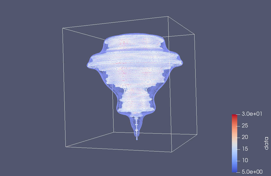
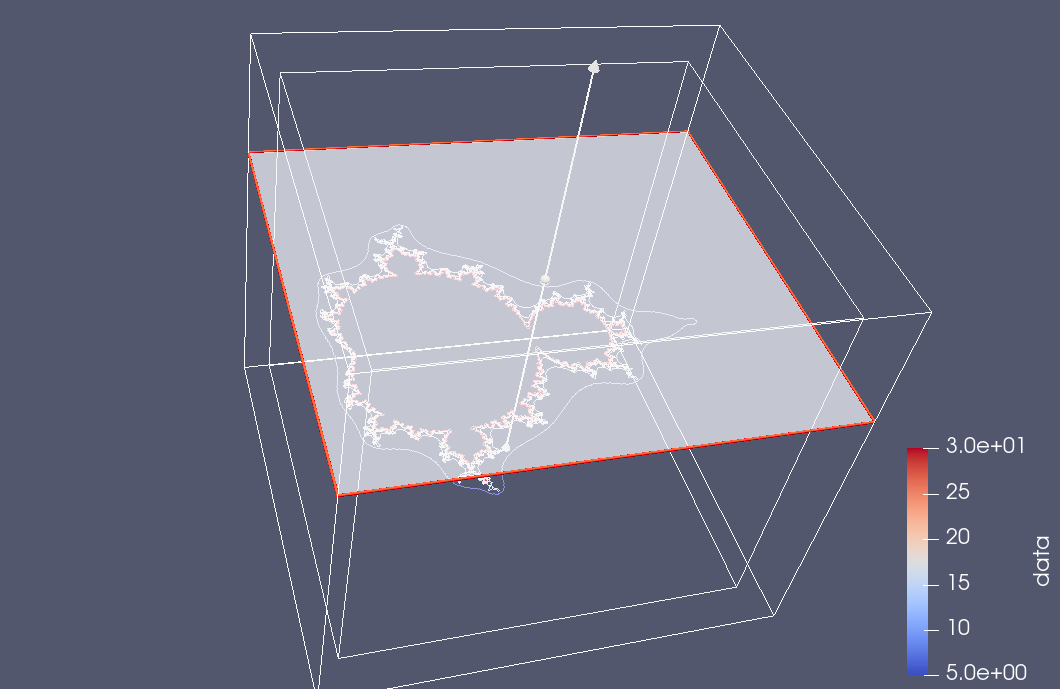
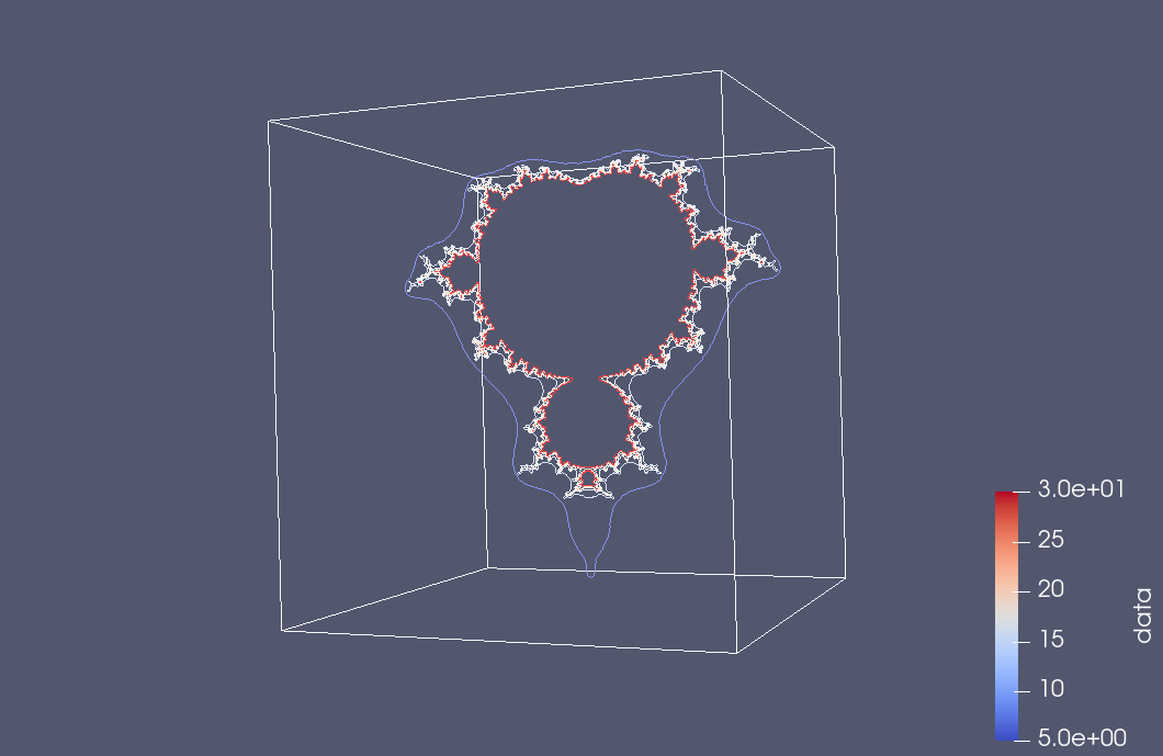
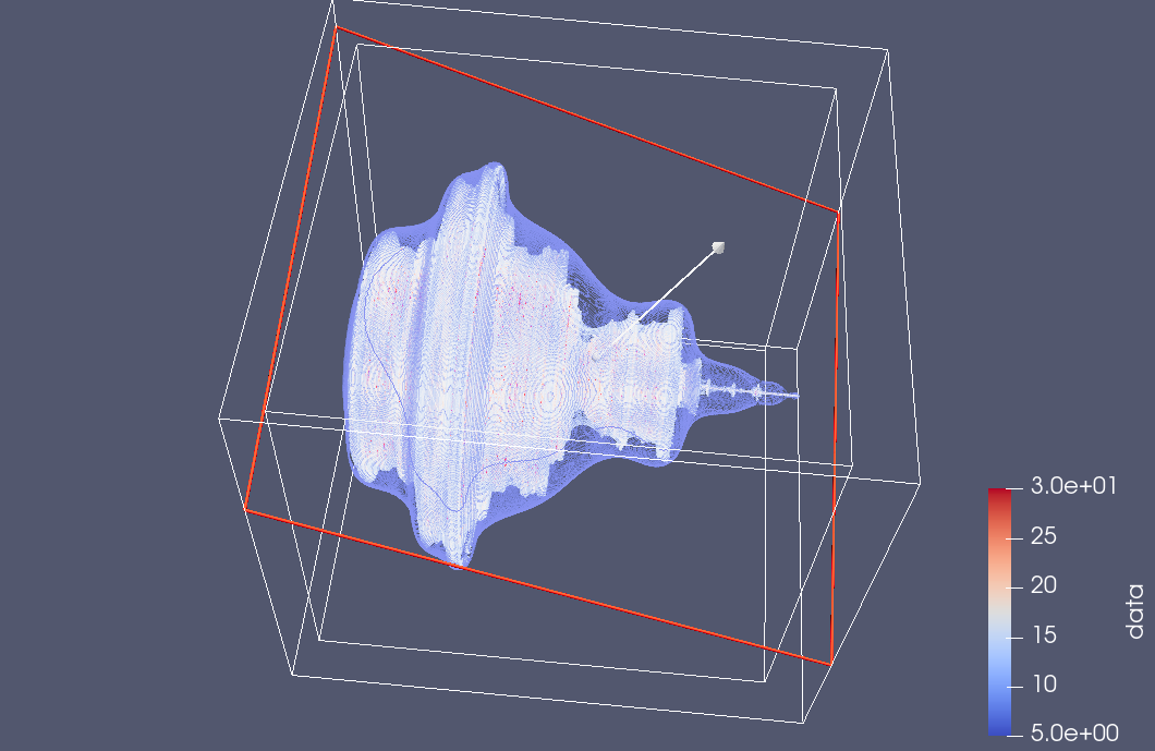
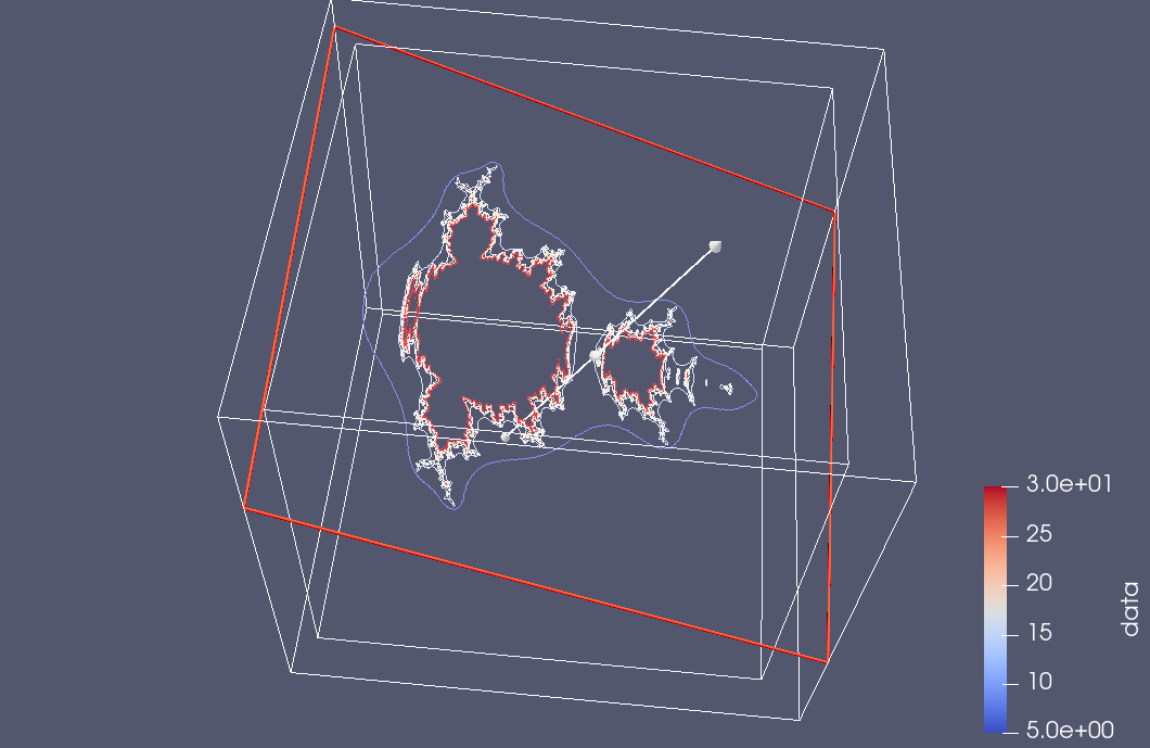
here is a bit more experimentation with Paraview slice filtering. This time I saved all the point data with the escape time counts, and rendered it with a few different contours

The default slice filter places the plane in the x-y orientation:

but we can also tilt it in the Paraview render UI

and suppress the contour view to see just the slice

As a very GUI challenged user, I don’t find the interface particularly intuitive, but have at least figured out this one particular slicing task, which is kind of cool.  It’s impressive that the UI can drive interesting computational tasks without having to regenerate or reload any of the raw data itself.  This time I was using the MacOSX Paraview client, which is nicer looking than the Windows version, but has some weird glitches in the file dialogues.

Analysis.

The graphing play above shows some apparent rotational symmetry our vector equivalent to the Mandelbrot equation
\begin{equation}
\Bx \rightarrow \Bx \Be_1 \Bx + \Bc.
\end{equation}
It was not clear to me if this symmetry existed, as there were artifacts in the plots that made it appear that there was irregularity. However, some thought shows that this irregularity is strictly due to sampling error, and perhaps also due to limitations in the plotting software, as such an uneven surface is probably tricky to deal with.

To see this, here are the first few iterations of the Mandlebrot sequence for an arbitary starting vector \( \Bc \).
\begin{equation}
\begin{aligned}
\Bx_0 &= \Bc \\
\Bx_1 &= \Bc \Be_1 \Bc + \Bc \\
\Bx_2 &= \lr{ \Bc \Be_1 \Bc + \Bc } \Be_1 \lr{ \Bc \Be_1 \Bc + \Bc } + \Bc \Be_1 \Bc + \Bc.
\end{aligned}
\end{equation}

Now, what happens when we rotate the starting vector \( \Bc \) in the \( y-z \) plane. The rotor for such a rotation is
\begin{equation}
R = \exp\lr{ e_{23} \theta/2 },
\end{equation}
where
\begin{equation}
\Bc \rightarrow R \Bc \tilde{R}.
\end{equation}
Observe that if \( \Bc \) is parallel to the x-axis, then this rotation leaves the starting point invariant, as \( \Be_1 \) commutes with \( R \). That is
\begin{equation}
R \Be_1 \tilde{R} =
\Be_1 R \tilde{R} = \Be_1.
\end{equation}
Let \( \Bc’ = R \Bc \tilde{R} \), so that
\begin{equation}
\Bx_0′ = R \Bc \tilde{R} = R \Bx_0 \tilde{R} .
\end{equation}
\begin{equation}
\begin{aligned}
\Bx_1′
&= R \Bc \tilde{R} \Be_1 R \Bc \tilde{R} + R \Bc \tilde{R} \\
&= R \Bc \Be_1 \Bc \tilde{R} + R \Bc \tilde{R} \\
&= R \lr{ \Bc \Be_1 \Bc R + \Bc } \tilde{R} \\
&= R \Bx_1 \tilde{R}.
\end{aligned}
\end{equation}
\begin{equation}\label{eqn:m2:n}
\begin{aligned}
\Bx_2′
&= \Bx_1′ \Be_1 \Bx_1′ + \Bc’ \\
&= R \Bx_1 \tilde{R} \Be_1 R \Bx_1 \tilde{R} + R \Bc \tilde{R} \\
&= R \Bx_1 \Be_1 \Bx_1 \tilde{R} + R \Bc \tilde{R} \\
&= R \lr{ \Bx_1 \Be_1 \Bx_1 + \Bc } \tilde{R} \\
&= R \Bx_2 \tilde{R}.
\end{aligned}
\end{equation}

The pattern is clear. If we rotate the starting point in the y-z plane, iterating the Mandelbrot sequence results in precisely the same rotation of the x-y plane Mandelbrot sequence. So the apparent rotational symmetry in the 3D iteration of the Mandelbrot vector equation is exactly that. This is an unfortunately boring 3D fractal. All of the interesting fractal nature occurs in the 2D plane, and the rest is just a consequence of rotating that image around the x-axis. We get some interesting fractal artifacts if we slice the rotated Mandelbrot image.

Some 3D renderings of the Mandelbrot set.

February 7, 2021 math and physics play , , , , ,

As mentioned previously, using geometric algebra we can convert the iterative equation for the Mandelbrot set from complex number form
\begin{equation}
z \rightarrow z^2 + c,
\end{equation}
to an equivalent vector form
\begin{equation}
\mathbf{x} \rightarrow \mathbf{x} \mathbf{e} \mathbf{x} + \mathbf{c},
\end{equation}
where \( \mathbf{e} \) represents the x-axis (say). Geometrically, each iteration takes \( \mathbf{e} \) and reflects it about the direction of \( \mathbf{x} \), then scales that by \( \mathbf{x}^2 \) and adds \( \mathbf{c} \).

To get the usual 2D Mandelbrot set, one iterates with vectors that lie only in the x-y plane, but we can treat the Mandelbrot set as a 3D solid if we remove the x-y plane restriction.

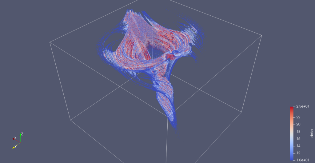
Last time I animated slices of the 3D set, but after a whole lot of messing around I managed to save the data for all the interior points of the 3D set in netCDF format, and render the solid using Paraview. Paraview has tons of filters available, and experimenting with them is pretty time consuming, but here are some initial screenshots of the 3D Mandelbrot set:

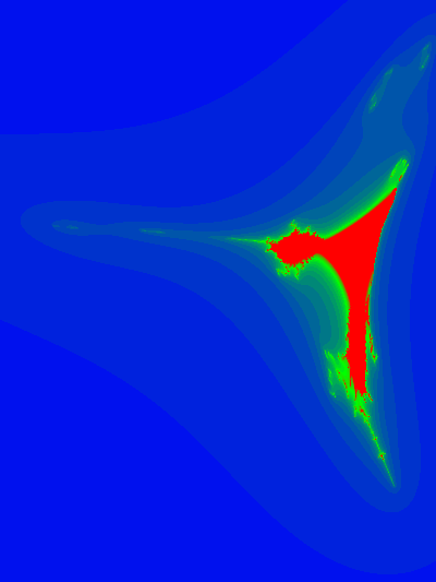
It’s interesting that much of the characteristic detail of the Mandelbrot set is not visible in the 3D volume, but if we slice that volume, you can then you can see it again.  Here’s a slice taken close to the z=0 plane (but far enough that the “CN tower” portion of the set is not visible)

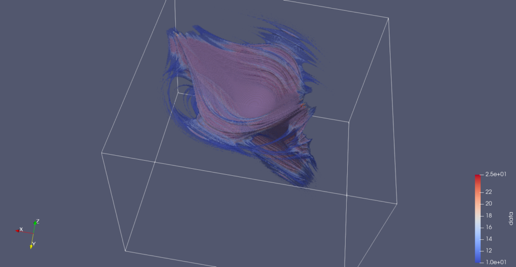
You can also see some of that detail if the opacity of the rendering is turned way down:

If you look carefully at the images above, you’ll see that the axis labels are wrong.  I think that I’ve screwed up one of the stride related parameters to my putVar call, and I end up with x+z transposed in the axes labels when visualized.

Visualizing the 3D Mandelbrot set.

February 1, 2021 C/C++ development and debugging.

In “Geometric Algebra for Computer Science” is a fractal problem based on a vectorization of the Mandelbrot equation, which allows for generalization to \( N \) dimensions.

I finally got around to trying the 3D variation of this problem.  Recall that the Mandlebrot set is a visualization of iteration of the following complex number equation:
\begin{equation}
z \rightarrow z^2 + c,
\end{equation}
where the idea is that \( z \) starts as the constant \( c \), and if this sequence converges to zero, then the point \( c \) is in the set.

The idea in the problem is that this equation can be cast as a vector equation, instead of a complex number equation. All we have to do is set \( z = \Be_1 \Bx \), where \( \Be_1 \) is the x-axis unit vector, and \( \Bx \) is an \(\mathbb{R}^2\) vector. Expanding in coordinates, with \( \Bx = \Be_1 x + \Be_2 y \), we have
\begin{equation}
z
= \Be_1 \lr{ \Be_1 x + \Be_2 y }
= x + \Be_1 \Be_2 y,
\end{equation}
but since the bivector \( \Be_1 \Be_2 \) squares to \( -1 \), we can represent complex numbers as even grade multivectors. Making the same substitution in the Mandlebrot equation, we have
\begin{equation}
\Be_1 \Bx \rightarrow \Be_1 \Bx \Be_1 \Bx + \Be_1 \Bc,
\end{equation}
or
\begin{equation}
\Bx \rightarrow \Bx \Be_1 \Bx + \Bc.
\end{equation}
Viola! This is a vector version of the Mandlebrot equation, and we can use it in 2 or 3 or N dimensions, as desired.  Observe that despite all the vector products above, the result is still a vector since \( \Bx \Be_1 \Bx \) is the geometric algebra form of a reflection of \( \Bx \) about the x-axis.

The problem with generalizing this from 2D is really one of visualization. How can we visualize a 3D Mandelbrot set? One idea I had was to use ray tracing, so that only the points on the surface from the desired viewpoint need be evaluated. I don’t think I’ve ever written a ray tracer, but I thought that there has got to be a quick and dirty way to do this.  Also, figuring out how to make a ray tracer interact with an irregular surface like this is probably non trivial!

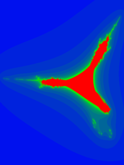
What I did instead, was a brute force evaluation of all the points in the upper half plane in around the origin, one slice of the set at a time. Here’s the result

Code for the visualization can be found in github. I’ve used Pauli matrices to do the evaluation, which is actually pretty quick (but slower than plain std::complex< double> evaluation), and the C++ ImageMagick API to save individual png files for the slices. There are better coloring schemes for the Mandelbrot set, and if I scrounge up some more time, I may try one of those instead.

Example of PL/I macro

January 27, 2021 Mainframe , , ,

Up until last week PL/I macros were a bit of a mystery.  Most of the ones that I’d seen in customer code were impressively inscrutable, and if I had to look at any of them, my reaction was to throw my hands in the air and plead with the compiler backend guys for help.  Implementing one such macro has been very helpful to understanding how these work.

Here is a C program that roughly models some PL/I code of interest

The documentation for the ‘foo’ function says of the final return code parameter that it is 12 bytes long, and that the ‘rcvalues.h’ header file has a set of RCNNN constants and a RCCHECK macro that can be used to test for any one of those constants.  A possible C implementation of that header might look something like:

/* rcvalues.h */
#define RC000 0x0000000000000000LL
#define RC001 0x0000000123456789LL
/* ... */

#define RCCHECK( urc, crc ) ( memcmp( &(urc), &(crc), 8 ) == 0 )

PL/I APIs do not typically use modern constructs like typedefs.  The closest that I have seen is for an API header file (copybook in the mainframe lingo) is to declare a variable (which becomes a local variable with a specific name in the including module), which the programmer can refer to using the LIKE keyword, as in the following example:

I believe there is also a DEFINE keyword available in newer PL/I compilers, which provides a typedef like mechanism, but most existing code probably doesn’t use such new-fangled nonsense, when cut and paste has far superior maintenance characteristics.  For that reason, the API would be unlikely to have a typedef equivalent for the return code structure.  Instead, the PL/I equivalent of the C code above, would probably look like:

(i.e. the C code is really modeled on the PL/I code of this form, and if this was a C API, the API would have a struct declaration or a typedef for the return code structure)

The RCNNN constants would actually be found as named variables (not immutable constants) in the copy book, perhaps declared something like:

I struggled a bit to figure out what the PL/I equivalent of my C RCCHECK macro would be.  The following inner function correctly did the required type casting and comparisons:

The implementation is very long, since the entire declaration of the input parameter type has to be duplicated.

If I was to put this RCCHECK implementation above into my RCVALUES.inc header file, it would only work if all the customer declaration of their return code structure objects were field by field compatible.  What I really want is for my RCCHECK function to take the address of the parameter, and pass that instead of the underlying type.  That was not at all obvious to figure out how to do, but with some help, I was eventually able to construct a PL/I macro (with helper inner-function) of the following form:

It’s clearly no longer a one liner.  Some notes on this PL/I macro:

  • The PL/I macro body looks like a regular PL/I function, but the begin-PROCEDURE and END statements start with % (% is not part of the PROC name.)
  • Macro parameters and return values are explicit strings, regardless of the types of the parameters that were actually passed.
  • In PL/I the || symbol is used for string concatenation, so this constructs output that inserts an ADDR() call around ARG1 token and then passes the ARG2 token as is.
  • I don’t know if there’s a way to implement this macro in a way that doesn’t require a helper function, and still have the output work in the context of an IF statement.
  • You have to explicitly enable the macro, using %ACTIVATE.  In my case, without %ACTIVATE, the RCCHECK symbol ends up as an undeclared external entry, and was no call to the @RCCHECK_HELPER function \({}^{[1]}\).
  • Observe that the PL/I macro provides a mechanism to jam whatever you want into the code, as the compiler’s macro preprocessor replaces the macro call tokens with the string that you have provided, leaving that string for the final compiler pass to interpret instead.

If I compile the code using this macro version of RCCHECK, the preprocessor output looks like:

I’m still pretty horrified at some of the macros that I’ve seen in customer code — they almost seem like the source equivalent of self modifying code.  You can’t figure out what is going on without also looking at all the output of the precompiler passes.  This is especially evil, since you can write PL/I preprocessor macros that generate preprocessor macros and require multiple preprocessor passes to produce the final desired output!

Footnotes

[1] note that @ is a valid PL/I character to use in a symbol name, as is # and $ — so if you want your functions to look like swear words, this is a language where that is possible.  Something like the following is probably valid PL/I :

V = #@$1A#@(1);

For added entertainment, your file names (i.e. PDS member names) can also be like ‘#@$1A#@’. Storing files with names like that on a Unix filesystem results in hours of fun, as you are then left with the task of figuring out how to properly quote file names with embedded $’s and #’s in scripts and makefiles.

Unpacking the fundamental theorem of multivector calculus in two dimensions

January 18, 2021 math and physics play , , , , , , , , , , , , , , , , , , ,

Notes.

Due to limitations in the MathJax-Latex package, all the oriented integrals in this blog post should be interpreted as having a clockwise orientation. [See the PDF version of this post for more sophisticated formatting.]

Guts.

Given a two dimensional generating vector space, there are two instances of the fundamental theorem for multivector integration
\begin{equation}\label{eqn:unpackingFundamentalTheorem:20}
\int_S F d\Bx \lrpartial G = \evalbar{F G}{\Delta S},
\end{equation}
and
\begin{equation}\label{eqn:unpackingFundamentalTheorem:40}
\int_S F d^2\Bx \lrpartial G = \oint_{\partial S} F d\Bx G.
\end{equation}
The first case is trivial. Given a parameterizated curve \( x = x(u) \), it just states
\begin{equation}\label{eqn:unpackingFundamentalTheorem:60}
\int_{u(0)}^{u(1)} du \PD{u}{}\lr{FG} = F(u(1))G(u(1)) – F(u(0))G(u(0)),
\end{equation}
for all multivectors \( F, G\), regardless of the signature of the underlying space.

The surface integral is more interesting. Let’s first look at the area element for this surface integral, which is
\begin{equation}\label{eqn:unpackingFundamentalTheorem:80}
d^2 \Bx = d\Bx_u \wedge d \Bx_v.
\end{equation}
Geometrically, this has the area of the parallelogram spanned by \( d\Bx_u \) and \( d\Bx_v \), but weighted by the pseudoscalar of the space. This is explored algebraically in the following problem and illustrated in fig. 1.

fig. 1. 2D vector space and area element.

Problem: Expansion of 2D area bivector.

Let \( \setlr{e_1, e_2} \) be an orthonormal basis for a two dimensional space, with reciprocal frame \( \setlr{e^1, e^2} \). Expand the area bivector \( d^2 \Bx \) in coordinates relating the bivector to the Jacobian and the pseudoscalar.

Answer

With parameterization \( x = x(u,v) = x^\alpha e_\alpha = x_\alpha e^\alpha \), we have
\begin{equation}\label{eqn:unpackingFundamentalTheorem:120}
\Bx_u \wedge \Bx_v
=
\lr{ \PD{u}{x^\alpha} e_\alpha } \wedge
\lr{ \PD{v}{x^\beta} e_\beta }
=
\PD{u}{x^\alpha}
\PD{v}{x^\beta}
e_\alpha
e_\beta
=
\PD{(u,v)}{(x^1,x^2)} e_1 e_2,
\end{equation}
or
\begin{equation}\label{eqn:unpackingFundamentalTheorem:160}
\Bx_u \wedge \Bx_v
=
\lr{ \PD{u}{x_\alpha} e^\alpha } \wedge
\lr{ \PD{v}{x_\beta} e^\beta }
=
\PD{u}{x_\alpha}
\PD{v}{x_\beta}
e^\alpha
e^\beta
=
\PD{(u,v)}{(x_1,x_2)} e^1 e^2.
\end{equation}
The upper and lower index pseudoscalars are related by
\begin{equation}\label{eqn:unpackingFundamentalTheorem:180}
e^1 e^2 e_1 e_2 =
-e^1 e^2 e_2 e_1 =
-1,
\end{equation}
so with \( I = e_1 e_2 \),
\begin{equation}\label{eqn:unpackingFundamentalTheorem:200}
e^1 e^2 = -I^{-1},
\end{equation}
leaving us with
\begin{equation}\label{eqn:unpackingFundamentalTheorem:140}
d^2 \Bx
= \PD{(u,v)}{(x^1,x^2)} du dv\, I
= -\PD{(u,v)}{(x_1,x_2)} du dv\, I^{-1}.
\end{equation}
We see that the area bivector is proportional to either the upper or lower index Jacobian and to the pseudoscalar for the space.

We may write the fundamental theorem for a 2D space as
\begin{equation}\label{eqn:unpackingFundamentalTheorem:680}
\int_S du dv \, \PD{(u,v)}{(x^1,x^2)} F I \lrgrad G = \oint_{\partial S} F d\Bx G,
\end{equation}
where we have dispensed with the vector derivative and use the gradient instead, since they are identical in a two parameter two dimensional space. Of course, unless we are using \( x^1, x^2 \) as our parameterization, we still want the curvilinear representation of the gradient \( \grad = \Bx^u \PDi{u}{} + \Bx^v \PDi{v}{} \).

Problem: Standard basis expansion of fundamental surface relation.

For a parameterization \( x = x^1 e_1 + x^2 e_2 \), where \( \setlr{ e_1, e_2 } \) is a standard (orthogonal) basis, expand the fundamental theorem for surface integrals for the single sided \( F = 1 \) case. Consider functions \( G \) of each grade (scalar, vector, bivector.)

Answer

From \ref{eqn:unpackingFundamentalTheorem:140} we see that the fundamental theorem takes the form
\begin{equation}\label{eqn:unpackingFundamentalTheorem:220}
\int_S dx^1 dx^2\, F I \lrgrad G = \oint_{\partial S} F d\Bx G.
\end{equation}
In a Euclidean space, the operator \( I \lrgrad \), is a \( \pi/2 \) rotation of the gradient, but has a rotated like structure in all metrics:
\begin{equation}\label{eqn:unpackingFundamentalTheorem:240}
I \grad
=
e_1 e_2 \lr{ e^1 \partial_1 + e^2 \partial_2 }
=
-e_2 \partial_1 + e_1 \partial_2.
\end{equation}

  • \( F = 1 \) and \( G \in \bigwedge^0 \) or \( G \in \bigwedge^2 \). For \( F = 1 \) and scalar or bivector \( G \) we have
    \begin{equation}\label{eqn:unpackingFundamentalTheorem:260}
    \int_S dx^1 dx^2\, \lr{ -e_2 \partial_1 + e_1 \partial_2 } G = \oint_{\partial S} d\Bx G,
    \end{equation}
    where, for \( x^1 \in [x^1(0),x^1(1)] \) and \( x^2 \in [x^2(0),x^2(1)] \), the RHS written explicitly is
    \begin{equation}\label{eqn:unpackingFundamentalTheorem:280}
    \oint_{\partial S} d\Bx G
    =
    \int dx^1 e_1
    \lr{ G(x^1, x^2(1)) – G(x^1, x^2(0)) }
    – dx^2 e_2
    \lr{ G(x^1(1),x^2) – G(x^1(0), x^2) }.
    \end{equation}
    This is sketched in fig. 2. Since a 2D bivector \( G \) can be written as \( G = I g \), where \( g \) is a scalar, we may write the pseudoscalar case as
    \begin{equation}\label{eqn:unpackingFundamentalTheorem:300}
    \int_S dx^1 dx^2\, \lr{ -e_2 \partial_1 + e_1 \partial_2 } g = \oint_{\partial S} d\Bx g,
    \end{equation}
    after right multiplying both sides with \( I^{-1} \). Algebraically the scalar and pseudoscalar cases can be thought of as identical scalar relationships.
  • \( F = 1, G \in \bigwedge^1 \). For \( F = 1 \) and vector \( G \) the 2D fundamental theorem for surfaces can be split into scalar
    \begin{equation}\label{eqn:unpackingFundamentalTheorem:320}
    \int_S dx^1 dx^2\, \lr{ -e_2 \partial_1 + e_1 \partial_2 } \cdot G = \oint_{\partial S} d\Bx \cdot G,
    \end{equation}
    and bivector relations
    \begin{equation}\label{eqn:unpackingFundamentalTheorem:340}
    \int_S dx^1 dx^2\, \lr{ -e_2 \partial_1 + e_1 \partial_2 } \wedge G = \oint_{\partial S} d\Bx \wedge G.
    \end{equation}
    To expand \ref{eqn:unpackingFundamentalTheorem:320}, let
    \begin{equation}\label{eqn:unpackingFundamentalTheorem:360}
    G = g_1 e^1 + g_2 e^2,
    \end{equation}
    for which
    \begin{equation}\label{eqn:unpackingFundamentalTheorem:380}
    \lr{ -e_2 \partial_1 + e_1 \partial_2 } \cdot G
    =
    \lr{ -e_2 \partial_1 + e_1 \partial_2 } \cdot
    \lr{ g_1 e^1 + g_2 e^2 }
    =
    \partial_2 g_1 – \partial_1 g_2,
    \end{equation}
    and
    \begin{equation}\label{eqn:unpackingFundamentalTheorem:400}
    d\Bx \cdot G
    =
    \lr{ dx^1 e_1 – dx^2 e_2 } \cdot \lr{ g_1 e^1 + g_2 e^2 }
    =
    dx^1 g_1 – dx^2 g_2,
    \end{equation}
    so \ref{eqn:unpackingFundamentalTheorem:320} expands to
    \begin{equation}\label{eqn:unpackingFundamentalTheorem:500}
    \int_S dx^1 dx^2\, \lr{ \partial_2 g_1 – \partial_1 g_2 }
    =
    \int
    \evalbar{dx^1 g_1}{\Delta x^2} – \evalbar{ dx^2 g_2 }{\Delta x^1}.
    \end{equation}
    This coordinate expansion illustrates how the pseudoscalar nature of the area element results in a duality transformation, as we end up with a curl like operation on the LHS, despite the dot product nature of the decomposition that we used. That can also be seen directly for vector \( G \), since
    \begin{equation}\label{eqn:unpackingFundamentalTheorem:560}
    dA (I \grad) \cdot G
    =
    dA \gpgradezero{ I \grad G }
    =
    dA I \lr{ \grad \wedge G },
    \end{equation}
    since the scalar selection of \( I \lr{ \grad \cdot G } \) is zero.In the grade-2 relation \ref{eqn:unpackingFundamentalTheorem:340}, we expect a pseudoscalar cancellation on both sides, leaving a scalar (divergence-like) relationship. This time, we use upper index coordinates for the vector \( G \), letting
    \begin{equation}\label{eqn:unpackingFundamentalTheorem:440}
    G = g^1 e_1 + g^2 e_2,
    \end{equation}
    so
    \begin{equation}\label{eqn:unpackingFundamentalTheorem:460}
    \lr{ -e_2 \partial_1 + e_1 \partial_2 } \wedge G
    =
    \lr{ -e_2 \partial_1 + e_1 \partial_2 } \wedge G
    \lr{ g^1 e_1 + g^2 e_2 }
    =
    e_1 e_2 \lr{ \partial_1 g^1 + \partial_2 g^2 },
    \end{equation}
    and
    \begin{equation}\label{eqn:unpackingFundamentalTheorem:480}
    d\Bx \wedge G
    =
    \lr{ dx^1 e_1 – dx^2 e_2 } \wedge
    \lr{ g^1 e_1 + g^2 e_2 }
    =
    e_1 e_2 \lr{ dx^1 g^2 + dx^2 g^1 }.
    \end{equation}
    So \ref{eqn:unpackingFundamentalTheorem:340}, after multiplication of both sides by \( I^{-1} \), is
    \begin{equation}\label{eqn:unpackingFundamentalTheorem:520}
    \int_S dx^1 dx^2\,
    \lr{ \partial_1 g^1 + \partial_2 g^2 }
    =
    \int
    \evalbar{dx^1 g^2}{\Delta x^2} + \evalbar{dx^2 g^1 }{\Delta x^1}.
    \end{equation}

As before, we’ve implicitly performed a duality transformation, and end up with a divergence operation. That can be seen directly without coordinate expansion, by rewriting the wedge as a grade two selection, and expanding the gradient action on the vector \( G \), as follows
\begin{equation}\label{eqn:unpackingFundamentalTheorem:580}
dA (I \grad) \wedge G
=
dA \gpgradetwo{ I \grad G }
=
dA I \lr{ \grad \cdot G },
\end{equation}
since \( I \lr{ \grad \wedge G } \) has only a scalar component.


fig. 2. Line integral around rectangular boundary.

Theorem 1.1: Green’s theorem [1].

Let \( S \) be a Jordan region with a piecewise-smooth boundary \( C \). If \( P, Q \) are continuously differentiable on an open set that contains \( S \), then
\begin{equation*}
\int dx dy \lr{ \PD{y}{P} – \PD{x}{Q} } = \oint P dx + Q dy.
\end{equation*}

Problem: Relationship to Green’s theorem.

If the space is Euclidean, show that \ref{eqn:unpackingFundamentalTheorem:500} and \ref{eqn:unpackingFundamentalTheorem:520} are both instances of Green’s theorem with suitable choices of \( P \) and \( Q \).

Answer

I will omit the subtleties related to general regions and consider just the case of an infinitesimal square region.

Start proof:

Let’s start with \ref{eqn:unpackingFundamentalTheorem:500}, with \( g_1 = P \) and \( g_2 = Q \), and \( x^1 = x, x^2 = y \), the RHS is
\begin{equation}\label{eqn:unpackingFundamentalTheorem:600}
\int dx dy \lr{ \PD{y}{P} – \PD{x}{Q} }.
\end{equation}
On the RHS we have
\begin{equation}\label{eqn:unpackingFundamentalTheorem:620}
\int \evalbar{dx P}{\Delta y} – \evalbar{ dy Q }{\Delta x}
=
\int dx \lr{ P(x, y_1) – P(x, y_0) } – \int dy \lr{ Q(x_1, y) – Q(x_0, y) }.
\end{equation}
This pair of integrals is plotted in fig. 3, from which we see that \ref{eqn:unpackingFundamentalTheorem:620} can be expressed as the line integral, leaving us with
\begin{equation}\label{eqn:unpackingFundamentalTheorem:640}
\int dx dy \lr{ \PD{y}{P} – \PD{x}{Q} }
=
\oint dx P + dy Q,
\end{equation}
which is Green’s theorem over the infinitesimal square integration region.

For the equivalence of \ref{eqn:unpackingFundamentalTheorem:520} to Green’s theorem, let \( g^2 = P \), and \( g^1 = -Q \). Plugging into the LHS, we find the Green’s theorem integrand. On the RHS, the integrand expands to
\begin{equation}\label{eqn:unpackingFundamentalTheorem:660}
\evalbar{dx g^2}{\Delta y} + \evalbar{dy g^1 }{\Delta x}
=
dx \lr{ P(x,y_1) – P(x, y_0)}
+
dy \lr{ -Q(x_1, y) + Q(x_0, y)},
\end{equation}
which is exactly what we found in \ref{eqn:unpackingFundamentalTheorem:620}.

End proof.


fig. 3. Path for Green’s theorem.

We may also relate multivector gradient integrals in 2D to the normal integral around the boundary of the bounding curve. That relationship is as follows.

Theorem 1.2: 2D gradient integrals.

\begin{equation*}
\begin{aligned}
\int J du dv \rgrad G &= \oint I^{-1} d\Bx G = \int J \lr{ \Bx^v du + \Bx^u dv } G \\
\int J du dv F \lgrad &= \oint F I^{-1} d\Bx = \int J F \lr{ \Bx^v du + \Bx^u dv },
\end{aligned}
\end{equation*}
where \( J = \partial(x^1, x^2)/\partial(u,v) \) is the Jacobian of the parameterization \( x = x(u,v) \). In terms of the coordinates \( x^1, x^2 \), this reduces to
\begin{equation*}
\begin{aligned}
\int dx^1 dx^2 \rgrad G &= \oint I^{-1} d\Bx G = \int \lr{ e^2 dx^1 + e^1 dx^2 } G \\
\int dx^1 dx^2 F \lgrad &= \oint G I^{-1} d\Bx = \int F \lr{ e^2 dx^1 + e^1 dx^2 }.
\end{aligned}
\end{equation*}
The vector \( I^{-1} d\Bx \) is orthogonal to the tangent vector along the boundary, and for Euclidean spaces it can be identified as the outwards normal.

Start proof:

Respectively setting \( F = 1 \), and \( G = 1\) in \ref{eqn:unpackingFundamentalTheorem:680}, we have
\begin{equation}\label{eqn:unpackingFundamentalTheorem:940}
\int I^{-1} d^2 \Bx \rgrad G = \oint I^{-1} d\Bx G,
\end{equation}
and
\begin{equation}\label{eqn:unpackingFundamentalTheorem:960}
\int F d^2 \Bx \lgrad I^{-1} = \oint F d\Bx I^{-1}.
\end{equation}
Starting with \ref{eqn:unpackingFundamentalTheorem:940} we find
\begin{equation}\label{eqn:unpackingFundamentalTheorem:700}
\int I^{-1} J du dv I \rgrad G = \oint d\Bx G,
\end{equation}
to find \( \int dx^1 dx^2 \rgrad G = \oint I^{-1} d\Bx G \), as desireed. In terms of a parameterization \( x = x(u,v) \), the pseudoscalar for the space is
\begin{equation}\label{eqn:unpackingFundamentalTheorem:720}
I = \frac{\Bx_u \wedge \Bx_v}{J},
\end{equation}
so
\begin{equation}\label{eqn:unpackingFundamentalTheorem:740}
I^{-1} = \frac{J}{\Bx_u \wedge \Bx_v}.
\end{equation}
Also note that \( \lr{\Bx_u \wedge \Bx_v}^{-1} = \Bx^v \wedge \Bx^u \), so
\begin{equation}\label{eqn:unpackingFundamentalTheorem:760}
I^{-1} = J \lr{ \Bx^v \wedge \Bx^u },
\end{equation}
and
\begin{equation}\label{eqn:unpackingFundamentalTheorem:780}
I^{-1} d\Bx
= I^{-1} \cdot d\Bx
= J \lr{ \Bx^v \wedge \Bx^u } \cdot \lr{ \Bx_u du – \Bx_v dv }
= J \lr{ \Bx^v du + \Bx^u dv },
\end{equation}
so the right acting gradient integral is
\begin{equation}\label{eqn:unpackingFundamentalTheorem:800}
\int J du dv \grad G =
\int
\evalbar{J \Bx^v G}{\Delta v} du + \evalbar{J \Bx^u G dv}{\Delta u},
\end{equation}
which we write in abbreviated form as \( \int J \lr{ \Bx^v du + \Bx^u dv} G \).

For the \( G = 1 \) case, from \ref{eqn:unpackingFundamentalTheorem:960} we find
\begin{equation}\label{eqn:unpackingFundamentalTheorem:820}
\int J du dv F I \lgrad I^{-1} = \oint F d\Bx I^{-1}.
\end{equation}
However, in a 2D space, regardless of metric, we have \( I a = – a I \) for any vector \( a \) (i.e. \( \grad \) or \( d\Bx\)), so we may commute the outer pseudoscalars in
\begin{equation}\label{eqn:unpackingFundamentalTheorem:840}
\int J du dv F I \lgrad I^{-1} = \oint F d\Bx I^{-1},
\end{equation}
so
\begin{equation}\label{eqn:unpackingFundamentalTheorem:850}
-\int J du dv F I I^{-1} \lgrad = -\oint F I^{-1} d\Bx.
\end{equation}
After cancelling the negative sign on both sides, we have the claimed result.

To see that \( I a \), for any vector \( a \) is normal to \( a \), we can compute the dot product
\begin{equation}\label{eqn:unpackingFundamentalTheorem:860}
\lr{ I a } \cdot a
=
\gpgradezero{ I a a }
=
a^2 \gpgradezero{ I }
= 0,
\end{equation}
since the scalar selection of a bivector is zero. Since \( I^{-1} = \pm I \), the same argument shows that \( I^{-1} d\Bx \) must be orthogonal to \( d\Bx \).

End proof.

Let’s look at the geometry of the normal \( I^{-1} \Bx \) in a couple 2D vector spaces. We use an integration volume of a unit square to simplify the boundary term expressions.

  • Euclidean: With a parameterization \( x(u,v) = u\Be_1 + v \Be_2 \), and Euclidean basis vectors \( (\Be_1)^2 = (\Be_2)^2 = 1 \), the fundamental theorem integrated over the rectangle \( [x_0,x_1] \times [y_0,y_1] \) is
    \begin{equation}\label{eqn:unpackingFundamentalTheorem:880}
    \int dx dy \grad G =
    \int
    \Be_2 \lr{ G(x,y_1) – G(x,y_0) } dx +
    \Be_1 \lr{ G(x_1,y) – G(x_0,y) } dy,
    \end{equation}
    Each of the terms in the integrand above are illustrated in fig. 4, and we see that this is a path integral weighted by the outwards normal.

    fig. 4. Outwards oriented normal for Euclidean space.

  • Spacetime: Let \( x(u,v) = u \gamma_0 + v \gamma_1 \), where \( (\gamma_0)^2 = -(\gamma_1)^2 = 1 \). With \( u = t, v = x \), the gradient integral over a \([t_0,t_1] \times [x_0,x_1]\) of spacetime is
    \begin{equation}\label{eqn:unpackingFundamentalTheorem:900}
    \begin{aligned}
    \int dt dx \grad G
    &=
    \int
    \gamma^1 dt \lr{ G(t, x_1) – G(t, x_0) }
    +
    \gamma^0 dx \lr{ G(t_1, x) – G(t_1, x) } \\
    &=
    \int
    \gamma_1 dt \lr{ -G(t, x_1) + G(t, x_0) }
    +
    \gamma_0 dx \lr{ G(t_1, x) – G(t_1, x) }
    .
    \end{aligned}
    \end{equation}
    With \( t \) plotted along the horizontal axis, and \( x \) along the vertical, each of the terms of this integrand is illustrated graphically in fig. 5. For this mixed signature space, there is no longer any good geometrical characterization of the normal.

    fig. 5. Orientation of the boundary normal for a spacetime basis.

  • Spacelike:
    Let \( x(u,v) = u \gamma_1 + v \gamma_2 \), where \( (\gamma_1)^2 = (\gamma_2)^2 = -1 \). With \( u = x, v = y \), the gradient integral over a \([x_0,x_1] \times [y_0,y_1]\) of this space is
    \begin{equation}\label{eqn:unpackingFundamentalTheorem:920}
    \begin{aligned}
    \int dx dy \grad G
    &=
    \int
    \gamma^2 dx \lr{ G(x, y_1) – G(x, y_0) }
    +
    \gamma^1 dy \lr{ G(x_1, y) – G(x_1, y) } \\
    &=
    \int
    \gamma_2 dx \lr{ -G(x, y_1) + G(x, y_0) }
    +
    \gamma_1 dy \lr{ -G(x_1, y) + G(x_1, y) }
    .
    \end{aligned}
    \end{equation}
    Referring to fig. 6. where the elements of the integrand are illustrated, we see that the normal \( I^{-1} d\Bx \) for the boundary of this region can be characterized as inwards.

    fig. 6. Inwards oriented normal for a Dirac spacelike basis.

References

[1] S.L. Salas and E. Hille. Calculus: one and several variables. Wiley New York, 1990.