forward Euler method

Final notes for ECE1254, Modelling of Multiphysics Systems

December 27, 2014 ece1254 , , , , , , , , , , , , , , , , , , , , , , , , , , , , , , , , , , , , , , , , , , , , , , , , , , , , , , , , , , , , , , , , , , , , ,

Capture

I’ve now finished my first grad course, Modelling of Multiphysics Systems, taught by Prof Piero Triverio.

I’ve posted notes for lectures and other material as I was taking the course, but now have an aggregated set of notes for the whole course posted.
This is now updated with all my notes from the lectures, solved problems, additional notes on auxillary topics I wanted to explore (like SVD), plus the notes from the Harmonic Balance report that Mike and I will be presenting in January.

This version of my notes also includes all the matlab figures regenerating using http://www.mathworks.com/matlabcentral/fileexchange/23629-export-fig, which allows a save-as pdf, which rescales much better than Matlab saveas() png’s when embedded in latex.  I’m not sure if that’s the best way to include Matlab figures in latex, but they are at least not fuzzy looking now.

All in all, I’m pretty pleased with my notes for this course.  They are a lot more readable than any of the ones I’ve done for the physics undergrad courses I was taking (https://peeterjoot.com/writing/).  While there was quite a lot covered in this course, the material really only requires an introductory circuits course and some basic math (linear algebra and intro calculus), so is pretty accessible.

This was a fun course.  I recall, back in ancient times when I was a first year student, being unsatisfied with all the ad-hoc strategies we used to solve circuits problems.  This finally answers the questions of how to tackle things more systematically.

Here’s the contents outline for these notes:

Preface
Lecture notes
1 nodal analysis
1.1 In slides
1.2 Mechanical structures example
1.3 Assembling system equations automatically. Node/branch method
1.4 Nodal Analysis
1.5 Modified nodal analysis (MNA)
2 solving large systems
2.1 Gaussian elimination
2.2 LU decomposition
2.3 Problems
3 numerical errors and conditioning
3.1 Strict diagonal dominance
3.2 Exploring uniqueness and existence
3.3 Perturbation and norms
3.4 Matrix norm
4 singular value decomposition, and conditioning number
4.1 Singular value decomposition
4.2 Conditioning number
5 sparse factorization
5.1 Fill ins
5.2 Markowitz product
5.3 Markowitz reordering
5.4 Graph representation
6 gradient methods
6.1 Summary of factorization costs
6.2 Iterative methods
6.3 Gradient method
6.4 Recap: Summary of Gradient method
6.5 Conjugate gradient method
6.6 Full Algorithm
6.7 Order analysis
6.8 Conjugate gradient convergence
6.9 Gershgorin circle theorem
6.10 Preconditioning
6.11 Symmetric preconditioning
6.12 Preconditioned conjugate gradient
6.13 Problems
7 solution of nonlinear systems
7.1 Nonlinear systems
7.2 Richardson and Linear Convergence
7.3 Newton’s method
7.4 Solution of N nonlinear equations in N unknowns
7.5 Multivariable Newton’s iteration
7.6 Automatic assembly of equations for nonlinear system
7.7 Damped Newton’s method
7.8 Continuation parameters
7.9 Singular Jacobians
7.10 Struts and Joints, Node branch formulation
7.11 Problems
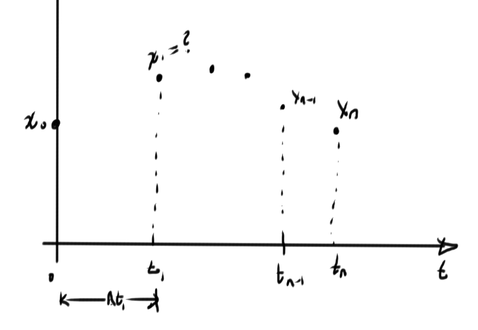
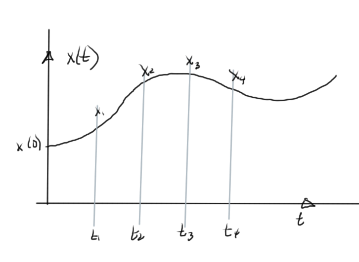
8 time dependent systems
8.1 Assembling equations automatically for dynamical systems
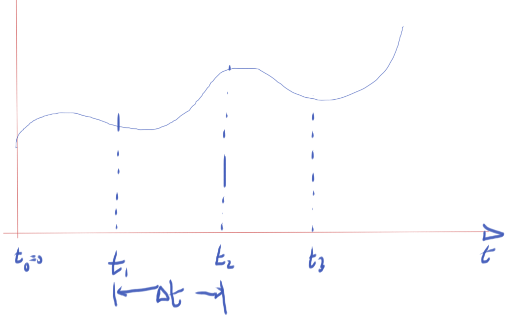
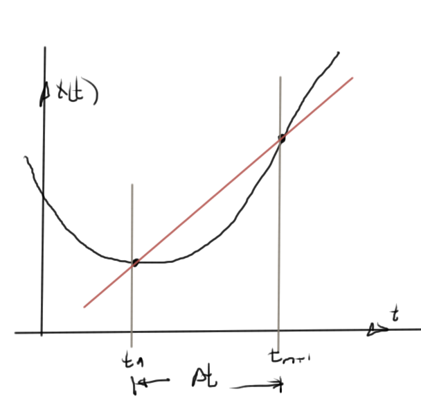
8.2 Numerical solution of differential equations
8.3 Forward Euler method
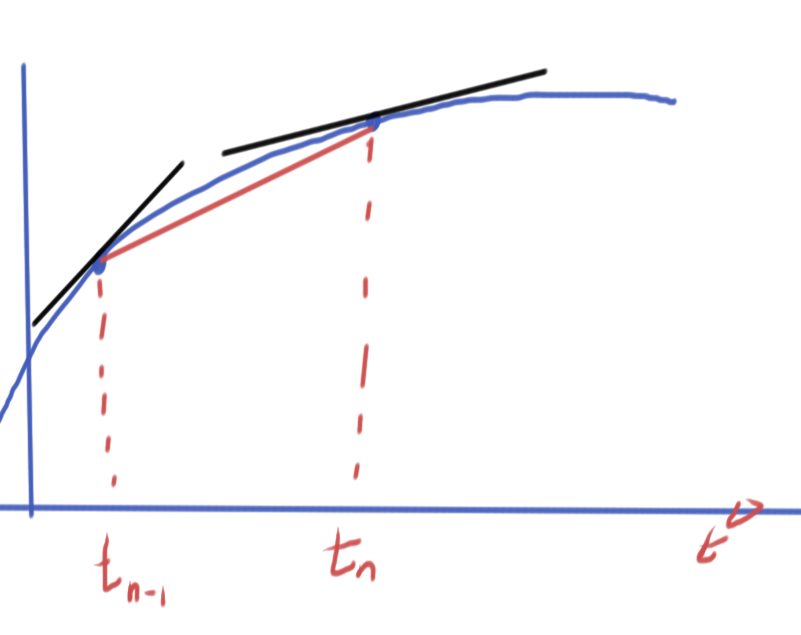
8.4 Backward Euler method
8.5 Trapezoidal rule (TR)
8.6 Nonlinear differential equations
8.7 Analysis, accuracy and stability (Dt ! 0)
8.8 Residual for LMS methods
8.9 Global error estimate
8.10 Stability
8.11 Stability (continued)
8.12 Problems
9 model order reduction
9.1 Model order reduction
9.2 Moment matching
9.3 Model order reduction (cont).
9.4 Moment matching
9.5 Truncated Balanced Realization (1000 ft overview)
9.6 Problems
Final report
10 harmonic balance
10.1 Abstract
10.2 Introduction
10.2.1 Modifications to the netlist syntax
10.3 Background
10.3.1 Discrete Fourier Transform
10.3.2 Harmonic Balance equations
10.3.3 Frequency domain representation of MNA equations
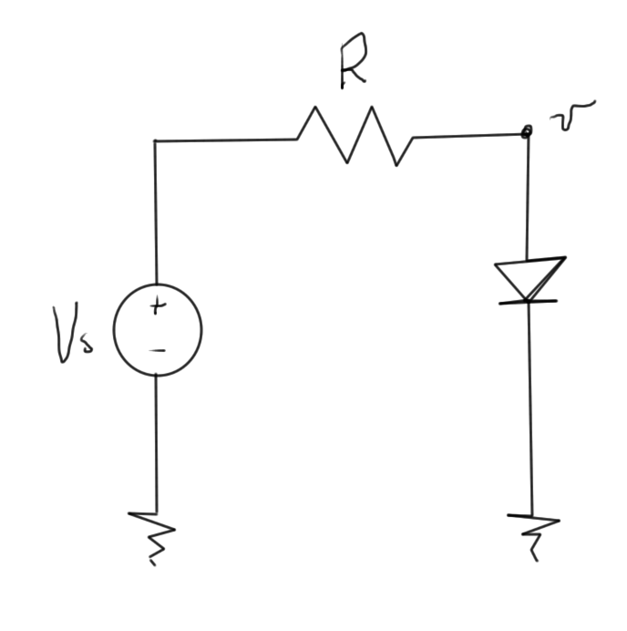
10.3.4 Example. RC circuit with a diode.
10.3.5 Jacobian
10.3.6 Newton’s method solution
10.3.7 Alternative handling of the non-linear currents and Jacobians
10.4 Results
10.4.1 Low pass filter
10.4.2 Half wave rectifier
10.4.3 AC to DC conversion
10.4.4 Bridge rectifier
10.4.5 Cpu time and error vs N
10.4.6 Taylor series non-linearities
10.4.7 Stiff systems
10.5 Conclusion
10.6 Appendices
10.6.1 Discrete Fourier Transform inversion
Appendices
a singular value decomposition
b basic theorems and definitions
c norton equivalents
d stability of discretized linear differential equations
e laplace transform refresher
f discrete fourier transform
g harmonic balance, rough notes
g.1 Block matrix form, with physical parameter ordering
g.2 Block matrix form, with frequency ordering
g.3 Representing the linear sources
g.4 Representing non-linear sources
g.5 Newton’s method
g.6 A matrix formulation of Harmonic Balance non-linear currents
h matlab notebooks
i mathematica notebooks
Index
Bibliography

ECE1254H Modeling of Multiphysics Systems. Lecture 15: Nonlinear differential equations. Taught by Prof. Piero Triverio

November 12, 2014 ece1254 , , , , , , , ,

[Click here for a PDF of this post with nicer formatting]

Disclaimer

Peeter’s lecture notes from class. These may be incoherent and rough.

Nonlinear differential equations

Assume that the relationships between the zeroth and first order derivatives has the form

\begin{equation}\label{eqn:multiphysicsL15:20}
F\lr{ x(t), \dot{x}(t) } = 0
\end{equation}
\begin{equation}\label{eqn:multiphysicsL15:40}
x(0) = x_0
\end{equation}

The backward Euler method where the derivative approximation is

\begin{equation}\label{eqn:multiphysicsL15:60}
\dot{x}(t_n) \approx \frac{x_n – x_{n-1}}{\Delta t},
\end{equation}

can be used to solve this numerically, reducing the problem to

\begin{equation}\label{eqn:multiphysicsL15:80}
F\lr{ x_n, \frac{x_n – x_{n-1}}{\Delta t} } = 0.
\end{equation}

This can be solved with Newton’s method. How do we find the initial guess for Newton’s? Consider a possible system in fig. 1.

lecture15Fig1

fig. 1. Possible solution points


One strategy for starting each iteration of Newton’s method is to base the initial guess for \( x_1 \) on the value \( x_0 \), and do so iteratively for each subsequent point. One can imagine that this may work up to some sample point \( x_n \), but then break down (i.e. Newton’s diverges when the previous value \( x_{n-1} \) is used to attempt to solve for \( x_n \)). At that point other possible strategies may work. One such strategy is to use an approximation of the derivative from the previous steps to attempt to get a better estimate of the next value. Another possibility is to reduce the time step, so the difference between successive points is reduced.

Analysis, accuracy and stability (\(\Delta t \rightarrow 0\))

Consider a differential equation

\begin{equation}\label{eqn:multiphysicsL15:100}
\dot{x}(t) = f(x(t), t)
\end{equation}
\begin{equation}\label{eqn:multiphysicsL15:120}
x(t_0) = x_0
\end{equation}

A few methods of solution have been considered

  • (FE) \( x_{n+1} – x_n = \Delta t f(x_n, t_n) \)
  • (BE) \( x_{n+1} – x_n = \Delta t f(x_{n+1}, t_{n+1}) \)
  • (TR) \( x_{n+1} – x_n = \frac{\Delta t}{2} f(x_{n+1}, t_{n+1}) + \frac{\Delta t}{2} f(x_{n}, t_{n}) \)

A common pattern can be observed, the generalization of which are called
\textit{linear multistep methods}
(LMS), which have the form

\begin{equation}\label{eqn:multiphysicsL15:140}
\sum_{j=-1}^{k-1} \alpha_j x_{n-j} = \Delta t \sum_{j=-1}^{k-1} \beta_j f( x_{n-j}, t_{n-j} )
\end{equation}

The FE (explicit), BE (implicit), and TR methods are now special cases with

  • (FE) \( \alpha_{-1} = 1, \alpha_0 = -1, \beta_{-1} = 0, \beta_0 = 1 \)
  • (BE) \( \alpha_{-1} = 1, \alpha_0 = -1, \beta_{-1} = 1, \beta_0 = 0 \)
  • (TR) \( \alpha_{-1} = 1, \alpha_0 = -1, \beta_{-1} = 1/2, \beta_0 = 1/2 \)

Here \( k \) is the number of timesteps used. The method is explicit if \( \beta_{-1} = 0 \).

Definition: Convergence

With

  • \(x(t)\) : exact solution
  • \(x_n\) : computed solution
  • \(e_n\) : where \( e_n = x_n – x(t_n) \), is the global error

The LMS method is convergent if

\begin{equation*}%\label{eqn:multiphysicsL15:180}
\max_{n, \Delta t \rightarrow 0} \Abs{ x_n – t(t_n) } \rightarrow 0 %\xrightarrow[t \rightarrow 0 ]{} 0
\end{equation*}

Convergence: zero-stability and consistency (small local errors made at each iteration),

where zero-stability is “small sensitivity to changes in initial condition”.

Definition: Consistency

A local error \( R_{n+1} \) can be defined as

\begin{equation*}%\label{eqn:multiphysicsL15:220}
R_{n+1} = \sum_{j = -1}^{k-1} \alpha_j x(t_{n-j}) – \Delta t \sum_{j=-1}^{k-1} \beta_j f(x(t_{n-j}), t_{n-j}).
\end{equation*}

The method is consistent if

\begin{equation*}%\label{eqn:multiphysicsL15:240}
\lim_{\Delta t} \lr{
\max_n \Abs{ \inv{\Delta t} R_{n+1} } = 0
}
\end{equation*}

or \( R_{n+1} \sim O({\Delta t}^2) \)

ECE1254H Modeling of Multiphysics Systems. Lecture 14: Backward Euler method and trapezoidal methods. Taught by Prof. Piero Triverio

November 10, 2014 ece1254 , , ,

[Click here for a PDF of this post with nicer formatting]

Disclaimer

Peeter’s lecture notes from class. These may be incoherent and rough.

Backward Euler method

Discretized time dependent partial differential equations were seen to have the form

\begin{equation}\label{eqn:multiphysicsL14:20}
G \Bx(t) + C \dot{\Bx}(t) = B \Bu(t),
\end{equation}

where \( G, C, B \) are matrices, and \( \Bu(t) \) is a vector of sources.

The backward Euler method augments \ref{eqn:multiphysicsL14:20} with an initial condition. For a one dimensional system such an initial condition could a zero time specification

\begin{equation}\label{eqn:multiphysicsL14:40}
G x(t) + C \dot{x}(t) = B u(t),
\end{equation}
\begin{equation}\label{eqn:multiphysicsL14:60}
x(0) = x_0
\end{equation}

Discretizing time as in fig. 1.

lecture14Fig1

fig. 1. Discretized time

The discrete derivative, using a backward difference, is

\begin{equation}\label{eqn:multiphysicsL14:80}
\dot{x}(t = t_n) \approx \frac{ x_n – x_{n-1} }{\Delta t}
\end{equation}

Evaluating \ref{eqn:multiphysicsL14:40} at \( t = t_n \) is

\begin{equation}\label{eqn:multiphysicsL14:100}
G x_n + C \dot{x}(t = t_n) = B u(t_n),
\end{equation}

or approximately

\begin{equation}\label{eqn:multiphysicsL14:120}
G x_n + C \frac{x_n – x_{n-1}}{\Delta t} = B u(t_n).
\end{equation}

Rearranging

\begin{equation}\label{eqn:multiphysicsL14:140}
\lr{ G + \frac{C}{\Delta t} } x_n = \frac{C}{\Delta t} x_{n-1}
+
B u(t_n).
\end{equation}

Assuming that matrices \( G, C \) are constant, and \( \Delta t \) is fixed, a matrix inversion can be avoided, and a single LU decomposition can be used. For \( N \) sampling points (not counting \( t_0 = 0 \)), \( N \) sets of backward and forward substitutions will be required to compute \( x_1 \) from \( x_0 \), and so forth.

Backwards Euler is an implicit method.

Recall that the forward Euler method gave

\begin{equation}\label{eqn:multiphysicsL14:160}
x_{n+1} =
x_n \lr{ I – C^{-1} \Delta t G }
+ C^{-1} \Delta t B u(t_n)
\end{equation}

This required

  • \( C \) must be invertible.
  • \( C \) must be cheap to invert, perhaps \( C = I \), so that
    \begin{equation}\label{eqn:multiphysicsL14:180}
    x_{n+1} =
    \lr{ I – \Delta t G } x_n
    + \Delta t B u(t_n)
    \end{equation}
  • This is an explicit method
  • This can be cheap but unstable.

Trapezoidal rule (TR)

The derivative can be approximated using an average of the pair of derivatives as illustrated in fig. 2.

lecture14Fig2

fig. 2. Trapezoidal derivative approximation

\begin{equation}\label{eqn:multiphysicsL14:200}
\frac{x_n – x_{n-1}}{\Delta t} \approx \frac{
\dot{x}(t_{n-1})
+
\dot{x}(t_{n})
}
{2}.
\end{equation}

Application to \ref{eqn:multiphysicsL14:40} for \( t_{n-1}, t_n \) respectively gives

\begin{equation}\label{eqn:multiphysicsL14:220}
\begin{aligned}
G x_{n-1} + C \dot{x}(t_{n-1}) &= B u(t_{n-1}) \\
G x_{n} + C \dot{x}(t_{n}) &= B u(t_{n}) \\
\end{aligned}
\end{equation}

Averaging these

\begin{equation}\label{eqn:multiphysicsL14:240}
G \frac{ x_{n-1} + x_n }{2} + C
\frac{
\dot{x}(t_{n-1})
+\dot{x}(t_{n})
}{2}
= B
\frac{u(t_{n-1})
+
u(t_{n}) }{2},
\end{equation}

and inserting the trapezoidal approximation

\begin{equation}\label{eqn:multiphysicsL14:280}
G \frac{ x_{n-1} + x_n }{2}
+
C
\frac{
x_{n} –
x_{n-1}
}{\Delta t}
= B
\frac{u(t_{n-1})
+
u(t_{n}) }{2},
\end{equation}

and a final rearrangement yields

\begin{equation}\label{eqn:multiphysicsL14:260}
\boxed{
\lr{ G + \frac{2}{\Delta t} C } x_n
=

\lr{ G – \frac{2}{\Delta t} C } x_{n_1}
+ B
\lr{u(t_{n-1})
+
u(t_{n}) }.
}
\end{equation}

This is

  • also an implicit method.
  • requires LU of \( G – 2 C /\Delta t \).
  • more accurate than BE, for the same computational cost.

In all of these methods, accumulation of error is something to be very careful of, and in some cases such error accumulation can even be exponential.

This is effectively a way to introduce central differences. On the slides this is seen to be more effective at avoiding either artificial damping and error accumulation that can be seen in backwards and forwards Euler method respectively.

ECE1254H Modeling of Multiphysics Systems. Lecture 13: Continuation parameters and Simulation of dynamical systems. Taught by Prof. Piero Triverio

October 29, 2014 ece1254 , ,

[Click here for a PDF of this post with nicer formatting]

Disclaimer

Peeter’s lecture notes from class. These may be incoherent and rough.

Singular Jacobians

(mostly on slides)

There is the possiblity of singular Jacobians to consider. FIXME: not sure how this system represented that. Look on slides.

lecture13Fig1

fig. 1. Diode system that results in singular Jacobian

\begin{equation}\label{eqn:multiphysicsL13:20}
\tilde{f}(v(\lambda), \lambda) = i(v) – \inv{R}( v – \lambda V_s ) = 0.
\end{equation}

An alternate continuation scheme uses

\begin{equation}\label{eqn:multiphysicsL13:40}
\tilde{F}(\Bx(\lambda), \lambda) = \lambda F(\Bx(\lambda)) + (1-\lambda) \Bx(\lambda).
\end{equation}

This scheme has

\begin{equation}\label{eqn:multiphysicsL13:60}
\tilde{F}(\Bx(0), 0) = 0
\end{equation}
\begin{equation}\label{eqn:multiphysicsL13:80}
\tilde{F}(\Bx(1), 1) = F(\Bx(1)),
\end{equation}

and for one variable, easy to compute Jacobian at the origin, or the original Jacobian at \( \lambda = 1 \)

\begin{equation}\label{eqn:multiphysicsL13:100}
\PD{x}{\tilde{F}}(x(0), 0) = I
\end{equation}
\begin{equation}\label{eqn:multiphysicsL13:120}
\PD{x}{\tilde{F}}(x(1), 1) = \PD{x}{F}(x(1))
\end{equation}

Simulation of dynamical systems

Example high level system in fig. 2.

lecture13Fig2

fig. 2. Complex time dependent system

Assembling equations automatically for dynamical systems

RC circuit

To demonstrate the method by example consider the RC circuit fig. 3 which has time dependence that must be considered

lecture13Fig3

fig. 3. RC circuit

The unknowns are \( v_1(t), v_2(t) \).

The equations (KCLs) at each of the nodes are

  1. \(
    \frac{v_1(t)}{R_1}
    + C_1 \frac{dv_1}{dt}
    + \frac{v_1(t) – v_2(t)}{R_2}
    + C_2 \frac{d(v_1 – v_2)}{dt}
    – i_{s,1}(t) = 0
    \)
  2. \(
    \frac{v_2(t) – v_1(t)}{R_2}
    + C_2 \frac{d(v_2 – v_1)}{dt}
    + \frac{v_2(t)}{R_3}
    + C_3 \frac{dv_2}{dt}
    – i_{s,2}(t)
    = 0
    \)

This has the matrix form
\begin{equation}\label{eqn:multiphysicsL13:140}
\begin{bmatrix}
Z_1 + Z_2 & – Z_2 \\
-Z_2 & Z_2 + Z_3
\end{bmatrix}
\begin{bmatrix}
v_1(t) \\
v_2(t)
\end{bmatrix}
+
\begin{bmatrix}
C_1 + C_2 & -C_2 \\
– C_2 & C_2 + C_3
\end{bmatrix}
\begin{bmatrix}
\frac{dv_1(t)}{dt} \\
\frac{dv_2(t}{dt})
\end{bmatrix}
=
\begin{bmatrix}
1 & 0 \\
0 & 1
\end{bmatrix}
\begin{bmatrix}
i_{s,1}(t) \\
i_{s,2}(t)
\end{bmatrix}.
\end{equation}

Observe that the capacitor between node 2 and 1 is associated with a stamp of the form

\begin{equation}\label{eqn:multiphysicsL13:180}
\begin{bmatrix}
C_2 & -C_2 \\
-C_2 & C_2
\end{bmatrix},
\end{equation}

very much like the impedance stamps of the resistor node elements.

The RC circuit problem has the abstract form

\begin{equation}\label{eqn:multiphysicsL13:160}
G \Bx(t) + C \frac{d\Bx(t)}{dt} = B \Bu(t),
\end{equation}

which is more general than a state space equation of the form

\begin{equation}\label{eqn:multiphysicsL13:200}
\frac{d\Bx(t)}{dt} = A \Bx(t) + B \Bu(t).
\end{equation}

Such a system may be represented diagramatically as in fig. 4.

lecture13Fig4

fig. 4. State space system

The \( C \) factor in this capacitance system, is generally not invertable. For example, if consider a 10 node system with only one capacitor, for which \( C \) will be mostly zeros.
In a state space system, in all equations we have a derivative. All equations are dynamical.

The time dependent MNA system for the RC circuit above, contains a mix of dynamical and algebraic equations. This could, for example, be a pair of equations like

\begin{equation}\label{eqn:multiphysicsL13:240}
\frac{dx_1}{dt} + x_2 + 3 = 0
\end{equation}
\begin{equation}\label{eqn:multiphysicsL13:260}
x_1 + x_2 + 3 = 0
\end{equation}

How to handle inductors

A pair of nodes that contains an inductor element, as in fig. 5, has to be handled specially.

lecture13Fig5

fig. 5. Inductor configuration

The KCL at node 1 has the form

\begin{equation}\label{eqn:multiphysicsL13:280}
\cdots + i_L(t) + \cdots = 0,
\end{equation}

where

\begin{equation}\label{eqn:multiphysicsL13:300}
v_{n_1}(t) – v_{n_2}(t) = L \frac{d i_L}{dt}.
\end{equation}

It is possible to express this in terms of \( i_L \), the variable of interest

\begin{equation}\label{eqn:multiphysicsL13:320}
i_L(t) = \inv{L} \int_0^t \lr{ v_{n_1}(\tau) – v_{n_2}(\tau) } d\tau
+ i_L(0).
\end{equation}

Expressing the problem directly in terms of such integrals makes the problem harder to solve, since the usual differential equation toolbox cannot be used directly. An integro-differential toolbox would have to be developed. What can be done instead is to introduce an additional unknown for each inductor current derivative \( di_L/dt \), for which an additional MNA row is introduced for that inductor scaled voltage difference.

Numerical solution of differential equations

Consider the one variable system

\begin{equation}\label{eqn:multiphysicsL13:340}
G x(t) + C \frac{dx}{dt} = B u(t),
\end{equation}

given an initial condition \( x(0) = x_0 \). Imagine that this system has the solution sketched in fig. 6.

lecture13Fig6

fig. 6. Discrete time sampling

Very roughly, the steps for solution are of the form

  1. Discretize time
  2. Aim to find the solution at \( t_1, t_2, t_3, \cdots \)
  3. Use a finite difference formula to approximate the derivative.

There are various schemes that can be used to discretize, and compute the finite differences.

Forward Euler method

\index{forward Euler method}

One such scheme is to use the forward differences, as in fig. 7, to approximate the derivative

\begin{equation}\label{eqn:multiphysicsL13:360}
\dot{x}(t_n) \approx \frac{x_{n+1} – x_n}{\Delta t}.
\end{equation}

lecture13Fig7

fig. 7. Forward difference derivative approximation

Introducing this into \ref{eqn:multiphysicsL13:340} gives

\begin{equation}\label{eqn:multiphysicsL13:350}
G x_n + C \frac{x_{n+1} – x_n}{\Delta t} = B u(t_n),
\end{equation}

or

\begin{equation}\label{eqn:multiphysicsL13:380}
C x_{n+1} = \Delta t B u(t_n) – \Delta t G x_n + C x_n.
\end{equation}

The coefficient \( C \) must be invertable, and the next point follows immediately

\begin{equation}\label{eqn:multiphysicsL13:381}
x_{n+1} = \frac{\Delta t B}{C} u(t_n)
+ x_n \lr{ 1 – \frac{\Delta t G}{C} }.
\end{equation}