[Click here for a PDF of this post with nicer formatting]
Disclaimer
Peeter’s lecture notes from class. These may be incoherent and rough.
These are notes for the UofT course PHY1520, Graduate Quantum Mechanics, taught by Prof. Paramekanti, covering [1] chap. 3 content.
Addition of angular momenta
-
For orbital angular momentum
\begin{equation}\label{eqn:qmLecture16:20}
\begin{aligned}
\hat{\BL}_1 &= \hat{\Br}_1 \cross \hat{\Bp}_1 \\
\hat{\BL}_1 &= \hat{\Br}_1 \cross \hat{\Bp}_1,
\end{aligned}
\end{equation}We can show that it is true that
\begin{equation}\label{eqn:qmLecture16:40}
\antisymmetric{L_{1i} + L_{2i}}{L_{1j} + L_{2j}} =
i \Hbar \epsilon_{i j k} \lr{ L_{1k} + L_{2k} },
\end{equation}because the angular momentum of the independent particles commute. Given this is it fair to consider that the sum
\begin{equation}\label{eqn:qmLecture16:60}
\hat{\BL}_1 + \hat{\BL}_2
\end{equation}is also angular momentum.
-
Given \( \ket{l_1, m_1} \) and \( \ket{l_2, m_2} \), if a measurement is made of \( \hat{\BL}_1 + \hat{\BL}_2 \), what do we get?
Specifically, what do we get for
\begin{equation}\label{eqn:qmLecture16:80}
\lr{\hat{\BL}_1 + \hat{\BL}_2}^2,
\end{equation}and for
\begin{equation}\label{eqn:qmLecture16:100}
\lr{\hat{L}_{1z} + \hat{L}_{2z}}.
\end{equation}For the latter, we get
\begin{equation}\label{eqn:qmLecture16:120}
\lr{\hat{L}_{1z} + \hat{L}_{2z}}\ket{ l_1, m_1 ; l_2, m_2 }
=
\lr{ \Hbar m_1 + \Hbar m_2 } \ket{ l_1, m_1 ; l_2, m_2 }
\end{equation}Given
\begin{equation}\label{eqn:qmLecture16:140}
\hat{L}_{1z} + \hat{L}_{2z} = \hat{L}_z^{\textrm{tot}},
\end{equation}we find
\begin{equation}\label{eqn:qmLecture16:160}
\begin{aligned}
\antisymmetric{\hat{L}_z^{\textrm{tot}}}{\hat{\BL}_1^2} &= 0 \\
\antisymmetric{\hat{L}_z^{\textrm{tot}}}{\hat{\BL}_2^2} &= 0 \\
\antisymmetric{\hat{L}_z^{\textrm{tot}}}{\hat{\BL}_{1z}} &= 0 \\
\antisymmetric{\hat{L}_z^{\textrm{tot}}}{\hat{\BL}_{1z}} &= 0.
\end{aligned}
\end{equation}We also find
\begin{equation}\label{eqn:qmLecture16:180}
\begin{aligned}
\antisymmetric{(\hat{\BL}_1 + \hat{\BL}_2)^2}{\BL_1^2}
&=
\antisymmetric{\hat{\BL}_1^2 + \hat{\BL}_2^2 + 2 \hat{\BL}_1 \cdot
\hat{\BL}_2}{\BL_1^2} \\
&=
0,
\end{aligned}
\end{equation}but for
\begin{equation}\label{eqn:qmLecture16:200}
\begin{aligned}
\antisymmetric{(\hat{\BL}_1 + \hat{\BL}_2)^2}{\hat{L}_{1z}}
&=
\antisymmetric{\hat{\BL}_1^2 + \hat{\BL}_2^2 + 2 \hat{\BL}_1 \cdot
\hat{\BL}_2}{\hat{L}_{1z}} \\
&=
2 \antisymmetric{\hat{\BL}_1 \cdot \hat{\BL}_2}{\hat{L}_{1z}} \\
&\ne 0.
\end{aligned}
\end{equation}
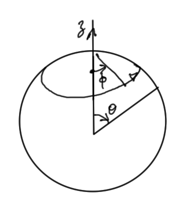
Classically if we have measured \( \hat{\BL}_{1} \) and \( \hat{\BL}_{2} \) then we know the total angular momentum as sketched in fig. 1.
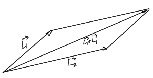
fig. 1. Classical addition of angular momenta.
In QM where we don’t know all the components of the angular momenum simultaneously, things get fuzzier. For example, if the \( \hat{L}_{1z} \) and \( \hat{L}_{2z} \) components have been measured, we have the angular momentum defined within a conical region as sketched in fig. 2.
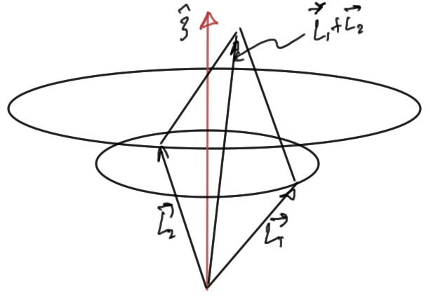
fig. 2. Addition of angular momenta given measured L_z
Suppose we know \( \hat{L}_z^{\textrm{tot}} \) precisely, but have impricise information about \( \lr{\hat{\BL}^{\textrm{tot}}}^2 \). Can we determine bounds for this? Let \( \ket{\psi} = \ket{ l_1, m_2 ; l_2, m_2 } \), so
\begin{equation}\label{eqn:qmLecture16:220}
\begin{aligned}
\bra{\psi} \lr{ \hat{\BL}_1 + \hat{\BL}_2 }^2 \ket{\psi}
&=
\bra{\psi} \hat{\BL}_1^2 \ket{\psi}
+ \bra{\psi} \hat{\BL}_2^2 \ket{\psi}
+ 2 \bra{\psi} \hat{\BL}_1 \cdot \hat{\BL}_2 \ket{\psi} \\
&=
l_1 \lr{ l_1 + 1} \Hbar^2
+ l_2 \lr{ l_2 + 1} \Hbar^2
+ 2
\bra{\psi} \hat{\BL}_1 \cdot \hat{\BL}_2 \ket{\psi}.
\end{aligned}
\end{equation}
Using the Cauchy-Schwartz inequality
\begin{equation}\label{eqn:qmLecture16:240}
\Abs{\braket{\phi}{\psi}}^2 \le
\Abs{\braket{\phi}{\phi}}
\Abs{\braket{\psi}{\psi}},
\end{equation}
which is the equivalent of the classical relationship
\begin{equation}\label{eqn:qmLecture16:260}
\lr{ \BA \cdot \BB }^2 \le \BA^2 \BB^2.
\end{equation}
Applying this to the last term, we have
\begin{equation}\label{eqn:qmLecture16:280}
\begin{aligned}
\lr{ \bra{\psi} \hat{\BL}_1 \cdot \hat{\BL}_2 \ket{\psi} }^2
&\le
\bra{ \psi} \hat{\BL}_1 \cdot \hat{\BL}_1 \ket{\psi}
\bra{ \psi} \hat{\BL}_2 \cdot \hat{\BL}_2 \ket{\psi} \\
&=
\Hbar^4
l_1 \lr{ l_1 + 1 }
l_2 \lr{ l_2 + 2 }.
\end{aligned}
\end{equation}
Thus for the max we have
\begin{equation}\label{eqn:qmLecture16:300}
\bra{\psi} \lr{ \hat{\BL}_1 + \hat{\BL}_2 }^2 \ket{\psi}
\le
\Hbar^2 l_1 \lr{ l_1 + 1 }
+\Hbar^2 l_2 \lr{ l_2 + 1 }
+ 2 \Hbar^2 \sqrt{ l_1 \lr{ l_1 + 1 } l_2 \lr{ l_2 + 2 } }
\end{equation}
and for the min
\begin{equation}\label{eqn:qmLecture16:360}
\bra{\psi} \lr{ \hat{\BL}_1 + \hat{\BL}_2 }^2 \ket{\psi}
\ge
\Hbar^2 l_1 \lr{ l_1 + 1 }
+\Hbar^2 l_2 \lr{ l_2 + 1 }
– 2 \Hbar^2 \sqrt{ l_1 \lr{ l_1 + 1 } l_2 \lr{ l_2 + 2 } }.
\end{equation}
To try to pretty up these estimate, starting with the max, note that if we replace a portion of the RHS with something bigger, we are left with a strict less than relationship.
That is
\begin{equation}\label{eqn:qmLecture16:320}
\begin{aligned}
l_1 \lr{ l_1 + 1 } &< \lr{ l_1 + \inv{2} }^2 \\
l_2 \lr{ l_2 + 1 } &< \lr{ l_2 + \inv{2} }^2
\end{aligned}
\end{equation}
That is
\begin{equation}\label{eqn:qmLecture16:340}
\begin{aligned}
\bra{\psi} \lr{ \hat{\BL}_1 + \hat{\BL}_2 }^2 \ket{\psi}
&<
\Hbar^2
\lr{
l_1 \lr{ l_1 + 1 }
+ l_2 \lr{ l_2 + 1 }
+ 2 \lr{ l_1 + \inv{2} } \lr{ l_2 + \inv{2} }
} \\
&=
\Hbar^2
\lr{
l_1^2 + l_2^2 + l_1 + l_2
+ 2 l_1 l_2 + l_1 + l_2 + \inv{2}
} \\
&=
\Hbar^2
\lr{
\lr{ l_1 + l_2 + \inv{2} }
\lr{ l_1 + l_2 + \frac{3}{2} } - \inv{4}
}
\end{aligned}
\end{equation}
or
\begin{equation}\label{eqn:qmLecture16:380}
l_{\textrm{tot}} \lr{ l_{\textrm{tot}} + 1 }
<
\lr{ l_1 + l_2 + \inv{2} }
\lr{ l_1 + l_2 + \frac{3}{2} }
,
\end{equation}
which, gives
\begin{equation}\label{eqn:qmLecture16:400}
l_{\textrm{tot}} < l_1 + l_2 + \inv{2}.
\end{equation}
Finally, given a quantization requirement, that is
\begin{equation}\label{eqn:t:1}
\boxed{
l_{\textrm{tot}} \le l_1 + l_2.
}
\end{equation}
Similarly, for the min, we find
\begin{equation}\label{eqn:qmLecture16:440}
\begin{aligned}
\bra{\psi} \lr{ \hat{\BL}_1 + \hat{\BL}_2 }^2 \ket{\psi}
&>
\Hbar^2
\lr{
l_1 \lr{ l_1 + 1 }
+ l_2 \lr{ l_2 + 1 }
– 2 \lr{ l_1 + \inv{2} } \lr{ l_2 + \inv{2} }
} \\
&=
\Hbar^2
\lr{
l_1^2 + l_2^2 %+ \cancel{l_1 + l_2}
– 2 l_1 l_2
– \inv{2}
}
\end{aligned}
\end{equation}
This will be finished Thursday, but we should get
\begin{equation}\label{eqn:t:2}
\boxed{
\Abs{l_1 – l_2} \le l_{\textrm{tot}} \le l_1 + l_2.
}
\end{equation}
References
[1] Jun John Sakurai and Jim J Napolitano. Modern quantum mechanics. Pearson Higher Ed, 2014.