spherical harmonics

Dipole field from multipole moment sum

November 12, 2016 math and physics play , , , , ,

[Click here for a PDF of this post with nicer formatting]

As indicated in Jackson [1], the components of the electric field can be obtained directly from the multipole moments

\begin{equation}\label{eqn:dipoleFromSphericalMoments:20}
\Phi(\Bx)
= \inv{4 \pi \epsilon_0} \sum \frac{4 \pi}{ (2 l + 1) r^{l + 1} } q_{l m} Y_{l m},
\end{equation}

so for the \( l,m \) contribution to this sum the components of the electric field are

\begin{equation}\label{eqn:dipoleFromSphericalMoments:40}
E_r
=
\inv{\epsilon_0} \sum \frac{l+1}{ (2 l + 1) r^{l + 2} } q_{l m} Y_{l m},
\end{equation}

\begin{equation}\label{eqn:dipoleFromSphericalMoments:60}
E_\theta
= -\inv{\epsilon_0} \sum \frac{1}{ (2 l + 1) r^{l + 2} } q_{l m} \partial_\theta Y_{l m}
\end{equation}

\begin{equation}\label{eqn:dipoleFromSphericalMoments:80}
\begin{aligned}
E_\phi
&= -\inv{\epsilon_0} \sum \frac{1}{ (2 l + 1) r^{l + 2} \sin\theta } q_{l m} \partial_\phi Y_{l m} \\
&= -\inv{\epsilon_0} \sum \frac{j m}{ (2 l + 1) r^{l + 2} \sin\theta } q_{l m} Y_{l m}.
\end{aligned}
\end{equation}

Here I’ve translated from CGS to SI. Let’s calculate the \( l = 1 \) electric field components directly from these expressions and check against the previously calculated results.

\begin{equation}\label{eqn:dipoleFromSphericalMoments:100}
\begin{aligned}
E_r
&=
\inv{\epsilon_0} \frac{2}{ 3 r^{3} }
\lr{
2 \lr{ -\sqrt{\frac{3}{8\pi}} }^2 \textrm{Re} \lr{
(p_x – j p_y) \sin\theta e^{j\phi}
}
+
\lr{ \sqrt{\frac{3}{4\pi}} }^2 p_z \cos\theta
} \\
&=
\frac{2}{4 \pi \epsilon_0 r^3}
\lr{
p_x \sin\theta \cos\phi + p_y \sin\theta \sin\phi + p_z \cos\theta
} \\
&=
\frac{1}{4 \pi \epsilon_0 r^3} 2 \Bp \cdot \rcap.
\end{aligned}
\end{equation}

Note that

\begin{equation}\label{eqn:dipoleFromSphericalMoments:120}
\partial_\theta Y_{11} = -\sqrt{\frac{3}{8\pi}} \cos\theta e^{j \phi},
\end{equation}

and

\begin{equation}\label{eqn:dipoleFromSphericalMoments:140}
\partial_\theta Y_{1,-1} = \sqrt{\frac{3}{8\pi}} \cos\theta e^{-j \phi},
\end{equation}

so

\begin{equation}\label{eqn:dipoleFromSphericalMoments:160}
\begin{aligned}
E_\theta
&=
-\inv{\epsilon_0} \frac{1}{ 3 r^{3} }
\lr{
2 \lr{ -\sqrt{\frac{3}{8\pi}} }^2 \textrm{Re} \lr{
(p_x – j p_y) \cos\theta e^{j\phi}
}

\lr{ \sqrt{\frac{3}{4\pi}} }^2 p_z \sin\theta
} \\
&=
-\frac{1}{4 \pi \epsilon_0 r^3}
\lr{
p_x \cos\theta \cos\phi + p_y \cos\theta \sin\phi – p_z \sin\theta
} \\
&=
-\frac{1}{4 \pi \epsilon_0 r^3} \Bp \cdot \thetacap.
\end{aligned}
\end{equation}

For the \(\phicap\) component, the \( m = 0 \) term is killed. This leaves

\begin{equation}\label{eqn:dipoleFromSphericalMoments:180}
\begin{aligned}
E_\phi
&=
-\frac{1}{\epsilon_0} \frac{1}{ 3 r^{3} \sin\theta }
\lr{
j q_{11} Y_{11} – j q_{1,-1} Y_{1,-1}
} \\
&=
-\frac{1}{3 \epsilon_0 r^{3} \sin\theta }
\lr{
j q_{11} Y_{11} – j (-1)^{2m} q_{11}^\conj Y_{11}^\conj
} \\
&=
\frac{2}{\epsilon_0} \frac{1}{ 3 r^{3} \sin\theta }
\textrm{Im} q_{11} Y_{11} \\
&=
\frac{2}{3 \epsilon_0 r^{3} \sin\theta }
\textrm{Im} \lr{
\lr{ -\sqrt{\frac{3}{8\pi}} }^2 (p_x – j p_y) \sin\theta e^{j \phi}
} \\
&=
\frac{1}{ 4 \pi \epsilon_0 r^{3} }
\textrm{Im} \lr{
(p_x – j p_y) e^{j \phi}
} \\
&=
\frac{1}{ 4 \pi \epsilon_0 r^{3} }
\lr{
p_x \sin\phi – p_y \cos\phi
} \\
&=
-\frac{\Bp \cdot \phicap}{ 4 \pi \epsilon_0 r^3}.
\end{aligned}
\end{equation}

That is
\begin{equation}\label{eqn:dipoleFromSphericalMoments:200}
\boxed{
\begin{aligned}
E_r &=
\frac{2}{4 \pi \epsilon_0 r^3}
\Bp \cdot \rcap \\
E_\theta &= –
\frac{1}{4 \pi \epsilon_0 r^3}
\Bp \cdot \thetacap \\
E_\phi &= –
\frac{1}{4 \pi \epsilon_0 r^3}
\Bp \cdot \phicap.
\end{aligned}
}
\end{equation}

These are consistent with equations (4.12) from the text for when \( \Bp \) is aligned with the z-axis.

Observe that we can sum each of the projections of \( \BE \) to construct the total electric field due to this \( l = 1 \) term of the multipole moment sum

\begin{equation}\label{eqn:dipoleFromSphericalMoments:n}
\begin{aligned}
\BE
&=
\frac{1}{4 \pi \epsilon_0 r^3}
\lr{
2 \rcap (\Bp \cdot \rcap)

\phicap ( \Bp \cdot \phicap)

\thetacap ( \Bp \cdot \thetacap)
} \\
&=
\frac{1}{4 \pi \epsilon_0 r^3}
\lr{
3 \rcap (\Bp \cdot \rcap)

\Bp
},
\end{aligned}
\end{equation}

which recovers the expected dipole moment approximation.

References

[1] JD Jackson. Classical Electrodynamics. John Wiley and Sons, 2nd edition, 1975.

PHY1520H Graduate Quantum Mechanics. Lecture 21: Non-degenerate perturbation. Taught by Prof. Arun Paramekanti

December 4, 2015 phy1520 , , ,

[Click here for a PDF of this post with nicer formatting]

Disclaimer

Peeter’s lecture notes from class. These may be incoherent and rough.

These are notes for the UofT course PHY1520, Graduate Quantum Mechanics, taught by Prof. Paramekanti, covering [2] chap. 5 content.

Non-degenerate perturbation theory. Recap.

\begin{equation}\label{eqn:qmLecture21:20}
\ket{n} = \ket{n_0}
+ \lambda \ket{n_1}
+ \lambda^2 \ket{n_2}
+ \lambda^3 \ket{n_3} + \cdots
\end{equation}

and

\begin{equation}\label{eqn:qmLecture21:40}
\Delta_{n} = \Delta_{n_0}
+ \lambda \Delta_{n_1}
+ \lambda^2 \Delta_{n_2}
+ \lambda^3 \Delta_{n_3} + \cdots
\end{equation}

\begin{equation}\label{eqn:qmLecture21:60}
\begin{aligned}
\Delta_{n_1} &= \bra{n^{(0)}} V \ket{n^{(0)}} \\
\ket{n_0} &= \ket{n^{(0)}}
\end{aligned}
\end{equation}

\begin{equation}\label{eqn:qmLecture21:80}
\begin{aligned}
\Delta_{n_2} &= \sum_{m \ne n} \frac{\Abs{\bra{n^{(0)}} V \ket{m^{(0)}}}^2}{E_n^{(0)} – E_m^{(0)}} \\
\ket{n_1} &= \sum_{m \ne n} \frac{ \ket{m^{(0)}} V_{mn} }{E_n^{(0)} – E_m^{(0)}}
\end{aligned}
\end{equation}

Example: Stark effect

\begin{equation}\label{eqn:qmLecture21:100}
H = H_{\textrm{atom}} + e \mathcal{E} z,
\end{equation}

where \( H_{\textrm{atom}} \) is assumed to be Hydrogen-like with Hamiltonian

\begin{equation}\label{eqn:qmLecture21:120}
H_{\textrm{atom}} = \frac{\BP^2}{2m} – \frac{e^2}{4 \pi \epsilon_0 r},
\end{equation}

and wave functions

\begin{equation}\label{eqn:qmLecture21:140}
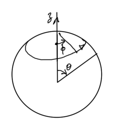
\braket{\Br}{\psi_{n l m}} = R_{n l}(r) Y_{lm}( \theta, \phi )
\end{equation}

For the first level correction to the energy

\begin{equation}\label{eqn:qmLecture21:160}
\begin{aligned}
\Delta_1
&= \bra{\psi_{100}} e \mathcal{E} z \ket{ \psi_{100}} \\
&= e \mathcal{E} \int \frac{d\Omega}{4 \pi} \cos \theta \int dr r^2 R_{100}^2(r)
\end{aligned}
\end{equation}

The cosine integral is obliterated, so we have \( \Delta_1 = 0 \).

How about the second order energy correction? That is

\begin{equation}\label{eqn:qmLecture21:180}
\Delta_2 = \sum_{n l m \ne 100} \frac{
\Abs{ \bra{\psi_{100}} e \mathcal{E} z \ket{ n l m }}^2
}{
E_{100}^{(0)} – E_{n l m}
}
\end{equation}

The matrix element in the numerator is the absolute square of

\begin{equation}\label{eqn:qmLecture21:200}
V_{100,nlm}
=
e \mathcal{E} \int d\Omega \inv{\sqrt{ 4 \pi } }
\cos\theta Y_{l m}(\theta, \phi)
\int dr r^3 R_{100}(r) R_{n l}(r).
\end{equation}

For all \( m \ne 0 \), \( Y_{lm} \) includes a \( e^{i m \phi} \) factor, so this cosine integral is zero. For \( m = 0 \), each of the \( Y_{lm} \) functions appears to contain either even or odd powers of cosines. For example:

\begin{equation}\label{eqn:qmLecture21:760}
\begin{aligned}
Y_{00} &= \frac{1}{2 \sqrt{\pi}} \\
Y_{10} &= \frac{1}{2} \sqrt{\frac{3}{\pi }} \cos(t) \\
Y_{20} &= \frac{1}{4} \sqrt{\frac{5}{\pi }} \lr{(3 \cos^2(t)-1} \\
Y_{30} &= \frac{1}{4} \sqrt{\frac{7}{\pi }} \lr{(5 \cos^3(t)-3 \cos(t)} \\
Y_{40} &= \frac{3 \lr{(35 \cos^4(t)-30 \cos^2(t)+3}}{16 \sqrt{\pi }} \\
Y_{50} &= \frac{1}{16} \sqrt{\frac{11}{\pi }} \lr{(63 \cos^5(t)-70 \cos^3(t)+15 \cos(t)} \\
Y_{60} &= \frac{1}{32} \sqrt{\frac{13}{\pi }} \lr{(231 \cos^6(t)-315 \cos^4(t)+105 \cos^2(t)-5} \\
Y_{70} &= \frac{1}{32} \sqrt{\frac{15}{\pi }} \lr{(429 \cos^7(t)-693 \cos^5(t)+315 \cos^3(t)-35 \cos(t)} \\
Y_{80} &= \frac{1}{256} \sqrt{\frac{17}{\pi }} \lr{(6435 \cos^8(t)-12012 \cos^6(t)+6930 \cos^4(t)-1260 \cos^2(t)+35 } \\
\end{aligned}
\end{equation}

This shows that for even \( 2k = l \), the cosine integral is zero

\begin{equation}\label{eqn:qmLecture21:780}
\int_0^\pi \sin\theta \cos\theta \sum_k a_k \cos^{2k}\theta d\theta
=
0,
\end{equation}

since \( \cos^{2k}(\theta) \) is even and \( \sin\theta \cos\theta \) is odd over the same interval. We find zero for \( \int_0^\pi \sin\theta \cos\theta Y_{30}(\theta, \phi) d\theta \), and Mathematica appears to show that the rest of these integrals for \( l > 1 \) are also zero.

FIXME: find the property of the spherical harmonics that can be used to prove that this is true in general for \( l > 1 \).

This leaves

\begin{equation}\label{eqn:qmLecture21:220}
\begin{aligned}
\Delta_2
&= \sum_{n \ne 1} \frac{
\Abs{ \bra{\psi_{100}} e \mathcal{E} z \ket{ n 1 0 }}^2
}{
E_{100}^{(0)} – E_{n 1 0}
} \\
&=
-e^2 \mathcal{E}^2
\sum_{n \ne 1} \frac{
\Abs{ \bra{\psi_{100}} z \ket{ n 1 0 }}^2
}{
E_{n 1 0}
-E_{100}^{(0)}
}.
\end{aligned}
\end{equation}

This is sometimes written in terms of a polarizability \( \alpha \)

\begin{equation}\label{eqn:qmLecture21:260}
\Delta_2 = -\frac{\mathcal{E}^2}{2} \alpha,
\end{equation}

where

\begin{equation}\label{eqn:qmLecture21:280}
\alpha =
2 e^2
\sum_{n \ne 1} \frac{
\Abs{ \bra{\psi_{100}} z \ket{ n 1 0 }}^2
}{
E_{n 1 0}
-E_{100}^{(0)}
}.
\end{equation}

With
\begin{equation}\label{eqn:qmLecture21:840}
\BP = \alpha \boldsymbol{\mathcal{E}},
\end{equation}

the energy change upon turning on the electric field from \( 0 \rightarrow \mathcal{E} \) is simply \( – \BP \cdot d\boldsymbol{\mathcal{E}} \) integrated from \( 0 \rightarrow \mathcal{E} \). Putting \( \BP = \alpha \mathcal{E} \zcap \), we have

\begin{equation}\label{eqn:qmLecture21:400}
\begin{aligned}
– \int_0^\mathcal{E} p_z d\mathcal{E}
&=
– \int_0^\mathcal{E} \alpha \mathcal{E} d\mathcal{E} \\
&=
– \inv{2} \alpha \mathcal{E}^2
\end{aligned}
\end{equation}

leading to an energy change \( – \alpha \mathcal{E}^2/2 \), so we can directly compute \( \expectation{\BP} \) or we can compute change in energy, and both contain information about the polarization factor \( \alpha \).

There is an exact answer to the sum \ref{eqn:qmLecture21:280}, but we aren’t going to try to get it here. Instead let’s look for bounds

\begin{equation}\label{eqn:qmLecture21:240}
\Delta_2^{\mathrm{min}} < \Delta_2 < \Delta_2^{\mathrm{max}}
\end{equation}

\begin{equation}\label{eqn:qmLecture21:320}
\alpha^{\mathrm{min}} = 2 e^2 \frac{
\Abs{ \bra{\psi_{100}} z \ket{\psi_{210}} }^2
}{E_{210}^{(0)} – E_{100}^{(0)}}
\end{equation}

For the hydrogen atom we have

\begin{equation}\label{eqn:qmLecture21:820}
E_n = -\frac{ e^2}{ 2 n^2 a_0 },
\end{equation}

allowing any difference of energy levels to be expressed as a fraction of the ground state energy, such as

\begin{equation}\label{eqn:qmLecture21:340}
E_{210}^{(0)} = \inv{4} E_{100}^{(0)} = \inv{4} \frac{ -\Hbar^2 }{ 2 m a_0^2 }
\end{equation}

So
\begin{equation}\label{eqn:qmLecture21:360}
E_{210}^{(0)} – E_{100}^{(0)} = \frac{3}{4}
\frac{ \Hbar^2 }{ 2 m a_0^2 }
\end{equation}

In the numerator we have

\begin{equation}\label{eqn:qmLecture21:380}
\begin{aligned}
\bra{\psi_{100}} z \ket{\psi_{210}}
&=
\int r^2 d\Omega
\lr{ \inv{\sqrt{\pi} a_0^{3/2}} e^{-r/a_0} } r \cos\theta \lr{
\inv{4 \sqrt{2 \pi} a_0^{3/2}} \frac{r}{a_0} e^{-r/2a_0} \cos\theta
} \\
&=
(2 \pi)
\inv{\sqrt{\pi}} \inv{4 \sqrt{2 \pi} } a_0
\int_0^\pi d\theta \sin\theta \cos^2\theta
\int_0^\infty \frac{dr}{a_0} \frac{r^4}{a_0^4} e^{-r/a_0 – r/2 a_0} \\
&=
(2 \pi)
\inv{\sqrt{\pi}} \inv{4 \sqrt{2 \pi} } a_0
\lr{ \evalrange{-\frac{u^3}{3}}{1}{-1} }
\int_0^\infty s^4 ds e^{- 3 s/2 } \\
&=
2
\inv{4 \sqrt{2} } a_0
\lr{ \evalrange{-\frac{u^3}{3}}{1}{-1} }
\int_0^\infty s^4 ds e^{- 3 s/2 } \\
&=
\inv{2 \sqrt{2}} \frac{2}{3} a_0 \frac{256}{81} \\
&=
\frac{1}{3 \sqrt{2} } \frac{ 256}{81} a_0
\approx 0.75 a_0.
\end{aligned}
\end{equation}

This gives

\begin{equation}\label{eqn:qmLecture21:420}
\begin{aligned}
\alpha^{\mathrm{min}}
&= \frac{ 2 e^2 (0.75)^2 a_0^2 }{ \frac{3}{4} \frac{\Hbar^2}{2 m a_0^2} } \\
&= \frac{6}{4} \frac{2 m e^2 a_0^4}{ \Hbar^2 } \\
&= 3 \frac{m e^2 a_0^4}{ \Hbar^2 } \\
&= 3 \frac{ 4 \pi \epsilon_0 }{a_0} a_0^4 \\
&\approx 4 \pi \epsilon_0 a_0^3 \times 3.
\end{aligned}
\end{equation}

The factor \( 4 \pi \epsilon_0 a_0^3 \) are the natural units for the polarizability.

There is a neat trick that generalizes to many problems to find the upper bound. Recall that the general polarizability was

\begin{equation}\label{eqn:qmLecture21:440}
\alpha
=
2 e^2
\sum_{nlm \ne 100} \frac{
\Abs{ \bra{100} z \ket{ n l m }}^2
}{
E_{n l m}
-E_{100}^{(0)}
}.
\end{equation}

If we are looking for the upper bound, and replace the denominator by the smallest energy difference that will be encountered, it can be brought out of the sum, for

\begin{equation}\label{eqn:qmLecture21:460}
\alpha^{\mathrm{max}} =
2 e^2
\inv{E_{2 1 0}
-E_{100}^{(0)} }
\sum_{nlm \ne 100}
\bra{100} z \ket{ n l m } \bra{nlm} z \ket{ 100 }
\end{equation}

Because \( \bra{nlm} z \ket{100} = 0 \), the constraint in the sum can be removed, and the identity summation evaluated

\begin{equation}\label{eqn:qmLecture21:480}
\begin{aligned}
\alpha^{\mathrm{max}}
&=
2 e^2
\inv{E_{2 1 0}
-E_{100}^{(0)} }
\sum_{nlm}
\bra{100} z \ket{ n l m } \bra{nlm} z \ket{ 100 } \\
&=
\frac{2 e^2 }{ \frac{3}{4} \frac{\Hbar^2}{ 2 m a_0^2} }
\bra{100} z^2 \ket{ 100 } \\
&=
\frac{16 e^2 m a_0^2 }{ 3 \Hbar^2 } \times a_0^2 \\
&=
4 \pi \epsilon_0 a_0^3 \times \frac{16}{3}.
\end{aligned}
\end{equation}

The bounds are

\begin{equation}\label{eqn:qmLecture21:520}
\boxed{
3 \ge \frac{\alpha}{\alpha^{\mathrm{at}}} < \frac{16}{3},
}
\end{equation}

where

\begin{equation}\label{eqn:qmLecture21:560}
\alpha^{\mathrm{at}} = 4 \pi \epsilon_0 a_0^3.
\end{equation}

The actual value is
\begin{equation}\label{eqn:qmLecture21:580}
\frac{\alpha}{\alpha^{\mathrm{at}}} = \frac{9}{2}.
\end{equation}

Example: Computing the dipole moment

\begin{equation}\label{eqn:qmLecture21:600}
\expectation{P_z}
= \alpha \mathcal{E}
= \bra{\psi_{100}} e z \ket{\psi_{100}}.
\end{equation}

Without any perturbation this is zero. After perturbation, retaining only the terms that are first order in \( \delta \psi_{100} \) we have

\begin{equation}\label{eqn:qmLecture21:620}
\bra{\psi_{100} + \delta \psi_{100}} e z \ket{\psi_{100} + \delta \psi_{100}}
\approx
\bra{\psi_{100}} e z \ket{\delta \psi_{100}}
+
\bra{\delta \psi_{100}} e z \ket{\psi_{100}}.
\end{equation}

Next time: Van der Walls

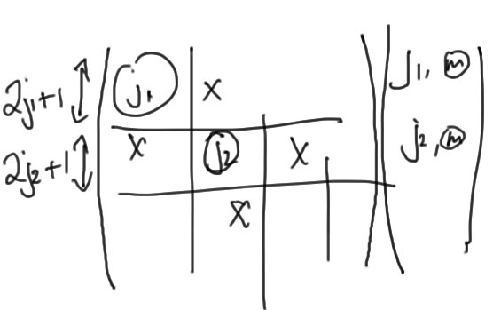
We will look at two hyrdogenic atomic systems interacting where the pair of nuclei are supposed to be infinitely heavy and stationary. The wave functions each set of atoms are individually known, but we can consider the problem of the interactions of atom 1’s electrons with atom 2’s nucleus and atom 2’s electrons, and also the opposite interactions of atom 2’s electrons with atom 1’s nucleus and its electrons. This leads to a result that is linear in the electric field (unlike the above result, which is called the quadratic Stark effect).

Appendix. Hydrogen wavefunctions

From [3], with the \( a_0 \) factors added in.

\begin{equation}\label{eqn:qmLecture21:660}
\psi_{1 s} = \psi_{100} = \inv{\sqrt{\pi} a_0^{3/2}} e^{-r/a_0}
\end{equation}
\begin{equation}\label{eqn:qmLecture21:680}
\psi_{2 s} = \psi_{200} = \inv{4 \sqrt{2 \pi} a_0^{3/2}} \lr{ 2 – \frac{r}{a_0} } e^{-r/2a_0}
\end{equation}
\begin{equation}\label{eqn:qmLecture21:700}
\psi_{2 p_x} = \inv{\sqrt{2}} \lr{ \psi_{2,1,1} – \psi_{2,1,-1} }
= \inv{4 \sqrt{2 \pi} a_0^{3/2}} \frac{r}{a_0} e^{-r/2a_0} \sin\theta\cos\phi
\end{equation}
\begin{equation}\label{eqn:qmLecture21:720}
\psi_{2 p_y} = \frac{i}{\sqrt{2}} \lr{ \psi_{2,1,1} + \psi_{2,1,-1} }
= \inv{4 \sqrt{2 \pi} a_0^{3/2}} \frac{r}{a_0} e^{-r/2a_0} \sin\theta\sin\phi
\end{equation}
\begin{equation}\label{eqn:qmLecture21:740}
\psi_{2 p_z} = \psi_{210} = \inv{4 \sqrt{2 \pi} a_0^{3/2}} \frac{r}{a_0} e^{-r/2a_0} \cos\theta
\end{equation}

I looked to [1] to see where to add in the \( a_0 \) factors.

References

[1] Carl R. Nave. Hydrogen Wavefunctions, 2015. URL http://hyperphysics.phy-astr.gsu.edu/hbase/quantum/hydwf.html. [Online; accessed 03-Dec-2015].

[2] Jun John Sakurai and Jim J Napolitano. Modern quantum mechanics. Pearson Higher Ed, 2014.

[3] Robert Field Troy Van Voorhis. Hydrogen Atom, 2013. URL https://ocw.mit.edu/courses/chemistry/5-61-physical-chemistry-fall-2013/lecture-notes/MIT5_61F13_Lecture19-20.pdf. [Online; accessed 03-Dec-2015].

PHY1520H Graduate Quantum Mechanics. Lecture 15: angular momentum rotation representation, and angular momentum addition. Taught by Prof. Arun Paramekanti

November 12, 2015 phy1520 , ,

[Click here for a PDF of this post with nicer formatting]

Disclaimer

Peeter’s lecture notes from class. These may be incoherent and rough.

These are notes for the UofT course PHY1520, Graduate Quantum Mechanics, taught by Prof. Paramekanti, covering chap 3. content from [1].

Angular momentum (wrap up.)

We found

\begin{equation}\label{eqn:qmLecture15:20}
\begin{aligned}
\hat{\BL^2} \ket{j, m} &= j(j+1) \Hbar^2 \ket{j,m} \\
\hat{L}_z \ket{j, m} &= \Hbar m \ket{j,m} \\
\hat{L}_{\pm} \ket{j, m } &= \Hbar \sqrt{(j \mp m)(j \pm m + 1)} \ket{j, m \pm 1 }
\end{aligned}
\end{equation}

or Schwinger

\begin{equation}\label{eqn:qmLecture15:40}
\begin{aligned}
\hat{L}_z &= \inv{2} \lr{ \hat{n}_1 – \hat{n}_2 } \Hbar \\
\hat{L}_{+} &= a_1^\dagger a_2 \Hbar \\
\hat{L}_{-} &= a_1 a_2^\dagger \Hbar \\
j &= \inv{2} \lr{ \hat{n}_1 + \hat{n}_2 },
\end{aligned}
\end{equation}

where each of the \( a_1, a_2 \) operators obey

\begin{equation}\label{eqn:qmLecture15:60}
\begin{aligned}
\antisymmetric{a_1}{a_1^\dagger} &= 1 \\
\antisymmetric{a_2}{a_2^\dagger} &= 1
\end{aligned}
\end{equation}

and any pair of different index \( a \) operators commute, as in

\begin{equation}\label{eqn:qmLecture15:80}
\antisymmetric{a_1}{a_2^\dagger} = 0.
\end{equation}

Representations

It’s possible to compute matrix representations of the rotation operators

\begin{equation}\label{eqn:qmLecture15:100}
\hat{R}_\ncap(\phi) = e^{i \hat{\BL} \cdot \ncap \phi/\Hbar}.
\end{equation}

With respect to a ket it’s possible to find

\begin{equation}\label{eqn:qmLecture15:120}
e^{i \hat{\BL} \cdot \ncap \phi/\Hbar} \ket{j, m}
=
\sum_{m’} d^j_{m m’}(\ncap, \phi) \ket{ j, m’ }.
\end{equation}

This has a block diagonal form that’s sketched in fig. 1.

fig. 1.  Block diagonal form for angular momentum matrix representation.

fig. 1. Block diagonal form for angular momentum matrix representation.

We can view \( d^j_{m m’}(\ncap, \phi) \) as a matrix, representing the rotation. The problem of determining these matrices can be reduced to that of determining the matrix for \( \hat{\BL} \), because once we have that we can exponentiate that.

Example: spin 1/2

From the eigenvalue relationships, with basis states

\begin{equation}\label{eqn:qmLecture15:160}
\begin{aligned}
\ket{\uparrow} &=
\begin{bmatrix}
1 \\
0
\end{bmatrix} \\
\ket{\downarrow} &=
\begin{bmatrix}
0 \\
1 \\
\end{bmatrix}
\end{aligned}
\end{equation}

we find

\begin{equation}\label{eqn:qmLecture15:180}
\begin{aligned}
\hat{L}_z &= \frac{\Hbar}{2} \begin{bmatrix} 1 & 0 \\ 0 & -1 \\ \end{bmatrix} \\
\hat{L}_{+} &= \frac{\Hbar}{2}
\begin{bmatrix}
0 & 1 \\
0 & 0
\end{bmatrix} \\
\hat{L}_{-} &= \frac{\Hbar}{2}
\begin{bmatrix}
0 & 0 \\
1 & 0
\end{bmatrix}.
\end{aligned}
\end{equation}

Rearranging we find the Pauli matrices

\begin{equation}\label{eqn:qmLecture15:200}
\hat{L}_k = \inv{2} \Hbar \sigma_i.
\end{equation}

Noting that \( \lr{ \Bsigma \cdot \ncap }^2 = 1 \), and \( \lr{\Bsigma \cdot \ncap }^3 = \Bsigma \cdot \ncap \), the rotation matrix is

\begin{equation}\label{eqn:qmLecture15:220}
e^{ i \Bsigma \cdot \ncap \phi/2 } \ket{\inv{2}, m} = \lr{ \cos( \phi/2 ) + i \Bsigma \cdot \ncap \sin(\phi/2) } \ket{\inv{2}, m}.
\end{equation}

The steps are

  1. Enumerate the states.
    \begin{equation}\label{eqn:qmLecture15:140}
    j_1 = \inv{2} \leftrightarrow\, \mbox{2 states (dimension of irrep = 2)}
    \end{equation}

  2. Construct the \( \hat{\BL} \) matrices.
  3. Construct \( d_{m m’}^j(\ncap, \phi) \).

Angular momentum operator in space representation

For \( L = 1 \) it turns out that the rotation matrices turn out to be the 3D rotation matrices. In the space representation

\begin{equation}\label{eqn:qmLecture15:240}
\BL = \Br \cross \Bp,
\end{equation}

the coordinates of the operator are

\begin{equation}\label{eqn:qmLecture15:260}
\hat{L}_k = i \epsilon_{k m n} r_m \lr{ -i \Hbar \PD{r_n}{} }
\end{equation}

We see that scaling \( \Br \rightarrow \alpha \Br \) does not change this operator, allowing for an angular representation \( \hat{L}_k(\theta, \phi) \) that have the form

\begin{equation}\label{eqn:qmLecture15:280}
\begin{aligned}
\hat{L}_z &= -i \Hbar \PD{\phi}{} \\
\hat{L}_{\pm} &= \Hbar \lr{ \pm \PD{\theta}{} + i \cot \theta \PD{\phi}{} }.
\end{aligned}
\end{equation}

Here \( \theta \) and \( \phi \) are the polar and azimuthal angles respectively as illustrated in fig. 2.

fig. 2.  Spherical coordinate convention.

fig. 2. Spherical coordinate convention.

The equivalent wave function representation of the problem is

\begin{equation}\label{eqn:qmLecture15:300}
\begin{aligned}
\hat{\BL} Y_{lm}(\theta, \phi) &= \Hbar^2 l (l + 1) Y_{lm}(\theta, \phi) \\
\hat{L}_z Y_{lm}(\theta, \phi) &= \Hbar m Y_{lm}(\theta, \phi) \\
\end{aligned}
\end{equation}

One can find these functions

\begin{equation}\label{eqn:qmLecture15:320}
Y_{lm}(\theta, \phi) = P_{l, m}(\cos \theta) e^{i m \phi},
\end{equation}

where \( P_{l, m}(\cos \theta) \) are called the associated Legendre polynomials. This can be applied whenever we have

\begin{equation}\label{eqn:qmLecture15:340}
\antisymmetric{H}{\hat{L}_k} = 0.
\end{equation}

where all the eigenfunctions will have the form

\begin{equation}\label{eqn:qmLecture15:360}
\Psi(r, \theta, \phi) = R(r) Y_{lm}(\theta, \phi).
\end{equation}

Addition of angular momentum

Since \( \hat{\BL} \) is a vector we expect to be able to add angular momentum in some way similar to the addition of classical vectors as illustrated in fig. 3.

fig. 3.  Classical vector addition.

fig. 3. Classical vector addition.

When we have a potential that depends only on the difference in position \( V(\Br_1 – \Br_2) \) then we know from classical problems it is effective to work in center of mass coordinates

\begin{equation}\label{eqn:qmLecture15:380}
\begin{aligned}
\hat{\BR}_{\textrm{cm}} &= \frac{\hat{\Br}_1 + \hat{\Br}_2}{2} \\
\hat{\BP}_{\textrm{cm}} &= \hat{\Bp}_1 + \hat{\Bp}_2
\end{aligned}
\end{equation}

where

\begin{equation}\label{eqn:qmLecture15:400}
\antisymmetric{\hat{R}_i}{\hat{P}_j} = i \Hbar \delta_{ij}.
\end{equation}

Given

\begin{equation}\label{eqn:qmLecture15:420}
\hat{\BL}_1 + \hat{\BL}_2 = \hat{\BL}_{\textrm{tot}},
\end{equation}

do we have
\begin{equation}\label{eqn:qmLecture15:440}
\antisymmetric{
\hat{L}_{\textrm{tot}, i}
}{
\hat{L}_{\textrm{tot}, j}
}
= i \Hbar \epsilon_{i j k} \hat{L}_{\textrm{tot}, k} ?
\end{equation}

That is

\begin{equation}\label{eqn:qmLecture15:460}
\antisymmetric{\hat{L}_{1,i} + \hat{L}_{1,j}}{\hat{L}_{2,i} + \hat{L}_{2,j}} = i \Hbar \epsilon_{i j k} \lr{ \hat{L}_{1,k} + \hat{L}_{1,k} }
\end{equation}

FIXME: Right at the end of the lecture, there was a mention of something about whether or not \( \hat{\BL}_1^2 \) and \( \hat{L}_{1,z} \) were sharply defined, but I missed it. Ask about this if not covered in the next lecture.

References

[1] Jun John Sakurai and Jim J Napolitano. Modern quantum mechanics. Pearson Higher Ed, 2014.

Update to old phy356 (Quantum Mechanics I) notes.

February 12, 2015 math and physics play , , , , , , , , , , , , , , , , , , , , , , , , , , , , , , , , , , , , , , , , , , , , , , , , , , , , , , , , , , , , , , , , , , , , , , , ,

It’s been a long time since I took QM I. My notes from that class were pretty rough, but I’ve cleaned them up a bit.

The main value to these notes is that I worked a number of introductory Quantum Mechanics problems.

These were my personal lecture notes for the Fall 2010, University of Toronto Quantum mechanics I course (PHY356H1F), taught by Prof. Vatche Deyirmenjian.

The official description of this course was:

The general structure of wave mechanics; eigenfunctions and eigenvalues; operators; orbital angular momentum; spherical harmonics; central potential; separation of variables, hydrogen atom; Dirac notation; operator methods; harmonic oscillator and spin.

This document contains a few things

• My lecture notes.
Typos, if any, are probably mine(Peeter), and no claim nor attempt of spelling or grammar correctness will be made. The first four lectures had chosen not to take notes for since they followed the text very closely.
• Notes from reading of the text. This includes observations, notes on what seem like errors, and some solved problems. None of these problems have been graded. Note that my informal errata sheet for the text has been separated out from this document.
• Some assigned problems. I have corrected some the errors after receiving grading feedback, and where I have not done so I at least recorded some of the grading comments as a reference.
• Some worked problems associated with exam preparation.