[Click here for a PDF of this post with nicer formatting]
Disclaimer
Peeter’s lecture notes from class. These may be incoherent and rough.
These are notes for the UofT course PHY1520, Graduate Quantum Mechanics, taught by Prof. Paramekanti, covering \textchapref{{1}} [1] content.
Coherent states (cont.)
A coherent state for the SHO \( H = \lr{ N + \inv{2} } \Hbar \omega \) was given by
\begin{equation}\label{eqn:qmLecture5:20}
a \ket{z} = z \ket{z},
\end{equation}
where we showed that
\begin{equation}\label{eqn:qmLecture5:40}
\ket{z} = c_0 e^{ z a^\dagger } \ket{0}.
\end{equation}
In the Heisenberg picture we found
\begin{equation}\label{eqn:qmLecture5:60}
\begin{aligned}
a_{\textrm{H}}(t) &= e^{i H t/\Hbar} a e^{-i H t/\Hbar} = a e^{-i\omega t} \\
a_{\textrm{H}}^\dagger(t) &= e^{i H t/\Hbar} a^\dagger e^{-i H t/\Hbar} = a^\dagger e^{i\omega t}.
\end{aligned}
\end{equation}
Recall that the position and momentum representation of the ladder operators was
\begin{equation}\label{eqn:qmLecture5:80}
\begin{aligned}
a &= \inv{\sqrt{2}} \lr{ \hat{x} \sqrt{\frac{m \omega}{\Hbar}} + i \hat{p} \sqrt{\inv{m \Hbar \omega}} } \\
a^\dagger &= \inv{\sqrt{2}} \lr{ \hat{x} \sqrt{\frac{m \omega}{\Hbar}} – i \hat{p} \sqrt{\inv{m \Hbar \omega}} },
\end{aligned}
\end{equation}
or equivalently
\begin{equation}\label{eqn:qmLecture5:100}
\begin{aligned}
\hat{x} &= \lr{ a + a^\dagger } \sqrt{\frac{\Hbar}{ 2 m \omega}} \\
\hat{p} &= i \lr{ a^\dagger – a } \sqrt{\frac{m \Hbar \omega}{2}}.
\end{aligned}
\end{equation}
Given this we can compute expectation value of position operator
\begin{equation}\label{eqn:qmLecture5:120}
\begin{aligned}
\bra{z} \hat{x} \ket{z}
&=
\sqrt{\frac{\Hbar}{ 2 m \omega}}
\bra{z}
\lr{ a + a^\dagger }
\ket{z} \\
&=
\lr{ z + z^\conj } \sqrt{\frac{\Hbar}{ 2 m \omega}} \\
&=
2 \textrm{Re} z \sqrt{\frac{\Hbar}{ 2 m \omega}} .
\end{aligned}
\end{equation}
Similarly
\begin{equation}\label{eqn:qmLecture5:140}
\begin{aligned}
\bra{z} \hat{p} \ket{z}
&=
i \sqrt{\frac{m \Hbar \omega}{2}}
\bra{z}
\lr{ a^\dagger – a }
\ket{z} \\
&=
\sqrt{\frac{m \Hbar \omega}{2}}
2 \textrm{Im} z.
\end{aligned}
\end{equation}
How about the expectation of the Heisenberg position operator? That is
\begin{equation}\label{eqn:qmLecture5:160}
\begin{aligned}
\bra{z} \hat{x}_{\textrm{H}}(t) \ket{z}
&=
\sqrt{\frac{\Hbar}{2 m \omega}} \bra{z} \lr{ a + a^\dagger } \ket{z} \\
&=
\sqrt{\frac{\Hbar}{2 m \omega}} \lr{ z e^{-i \omega t} + z^\conj e^{i \omega t}} \\
&=
\sqrt{\frac{\Hbar}{2 m \omega}} \lr{ \lr{z + z^\conj} \cos( \omega t ) -i \lr{ z – z^\conj } \sin( \omega t) } \\
&=
\sqrt{\frac{\Hbar}{2 m \omega}} \lr{ \expectation{x(0)} \sqrt{ \frac{2 m \omega}{\Hbar}} \cos( \omega t ) -i \expectation{p(0)} i \sqrt{\frac{2 m \omega}{\Hbar} } \sin( \omega t) } \\
&=
\expectation{x(0)} \cos( \omega t ) + \frac{\expectation{p(0)}}{m \omega} \sin( \omega t) .
\end{aligned}
\end{equation}
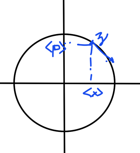
We find that the average of the Heisenberg position operator evolves in time in exactly the same fashion as position in the classical Harmonic oscillator. This phase space like trajectory is sketched in fig. 1.
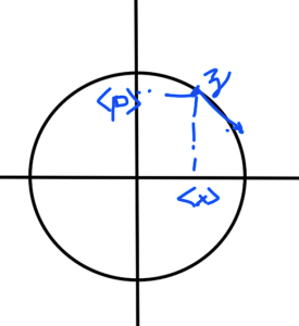
fig. 1. phase space like trajectory
In the text it is shown that we have the same structure for the Heisenberg operator itself, before taking expectations
\begin{equation}\label{eqn:qmLecture5:220}
\hat{x}_{\textrm{H}}(t)
=
{x(0)} \cos( \omega t ) + \frac{{p(0)}}{m \omega} \sin( \omega t).
\end{equation}
Where the coherent states become useful is that we will see that the second moments of position and momentum are not time dependent with respect to the coherent states. Such states remain localized.
Uncertainty
First note that using the commutator relationship we have
\begin{equation}\label{eqn:qmLecture5:180}
\begin{aligned}
\bra{z} a a^\dagger \ket{z}
&=
\bra{z} \lr{ \antisymmetric{a}{a^\dagger} + a^\dagger a } \ket{z} \\
&=
\bra{z} \lr{ 1 + a^\dagger a } \ket{z}.
\end{aligned}
\end{equation}
For the second moment we have
\begin{equation}\label{eqn:qmLecture5:200}
\begin{aligned}
\bra{z} \hat{x}^2 \ket{z}
&=
\frac{\Hbar}{ 2 m \omega}
\bra{z} \lr{a + a^\dagger } \lr{a + a^\dagger } \ket{z} \\
&=
\frac{\Hbar}{ 2 m \omega}
\bra{z} \lr{
a^2 + {(a^\dagger)}^2 + a a^\dagger + a^\dagger a
} \ket{z} \\
&=
\frac{\Hbar}{ 2 m \omega}
\bra{z} \lr{
a^2 + {(a^\dagger)}^2 + 2 a^\dagger a + 1
} \ket{z} \\
&=
\frac{\Hbar}{ 2 m \omega}
\lr{ z^2 + {(z^\conj)}^2 + 2 z^\conj z + 1} \ket{z} \\
&=
\frac{\Hbar}{ 2 m \omega}
\lr{ z + z^\conj }^2
+
\frac{\Hbar}{ 2 m \omega}.
\end{aligned}
\end{equation}
We find
\begin{equation}\label{eqn:qmLecture5:240}
\sigma_x^2 = \frac{\Hbar}{ 2 m \omega},
\end{equation}
and
\begin{equation}\label{eqn:qmLecture5:260}
\sigma_p^2 = \frac{m \Hbar \omega}{2}
\end{equation}
so
\begin{equation}\label{eqn:qmLecture5:280}
\sigma_x^2 \sigma_p^2 = \frac{\Hbar^2}{4},
\end{equation}
or
\begin{equation}\label{eqn:qmLecture5:300}
\sigma_x \sigma_p = \frac{\Hbar}{2}.
\end{equation}
This is the minimum uncertainty.
Quantum Field theory
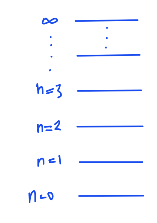
In Quantum Field theory the ideas of isolated oscillators is used to model particle creation. The lowest energy state (a no particle, vacuum state) is given the lowest energy level, with each additional quantum level modeling a new particle creation state as sketched in fig. 2.
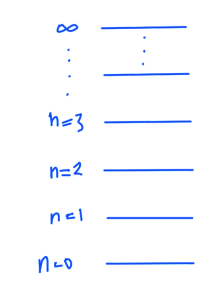
fig. 2. QFT energy levels
We have to imagine many oscillators, each with a distinct vacuum energy \( \sim \Bk^2 \) . The Harmonic oscillator can be used to model the creation of particles with \( \Hbar \omega \) energy differences from that “vacuum energy”.
Charged particle in a magnetic field
In the classical case ( with SI units or \( c = 1 \) ) we have
\begin{equation}\label{eqn:qmLecture5:320}
\BF = q \BE + q \Bv \cross \BB.
\end{equation}
Alternately, we can look at the Hamiltonian view of the system, written in terms of potentials
\begin{equation}\label{eqn:qmLecture5:340}
\BB = \spacegrad \cross \BA,
\end{equation}
\begin{equation}\label{eqn:qmLecture5:360}
\BE = – \spacegrad \phi – \PD{t}{\BA}.
\end{equation}
Note that the curl form for the magnetic field implies one of the required Maxwell’s equations \( \spacegrad \cdot \BB = 0 \).
Ignoring time dependence of the potentials, the Hamiltonian can be expressed as
\begin{equation}\label{eqn:qmLecture5:380}
H = \inv{2 m} \lr{ \Bp – q \BA }^2 + q \phi.
\end{equation}
In this Hamiltonian the vector \( \Bp \) is called the canonical momentum, the momentum conjugate to position in phase space.
It is left as an exercise to show that the Lorentz force equation results from application of the Hamiltonian equations of motion, and that the velocity is given by \( \Bv = (\Bp – q \BA)/m \).
For quantum mechanics, we use the same Hamiltonian, but promote our position, momentum and potentials to operators.
\begin{equation}\label{eqn:qmLecture5:400}
\hat{H} = \inv{2 m} \lr{ \hat{\Bp} – q \hat{\BA}(\Br, t) }^2 + q \hat{\phi}(\Br, t).
\end{equation}
Gauge invariance
Can we say anything about this before looking at the question of a particle in a magnetic field?
Recall that the we can make a gauge transformation of the form
\label{eqn:qmLecture5:420a}
\begin{equation}\label{eqn:qmLecture5:420}
\BA \rightarrow \BA + \spacegrad \chi
\end{equation}
\begin{equation}\label{eqn:qmLecture5:440}
\phi \rightarrow \phi – \PD{t}{\chi}
\end{equation}
Does this notion of gauge invariance also carry over to the Quantum Hamiltonian. After gauge transformation we have
\begin{equation}\label{eqn:qmLecture5:460}
\hat{H}’
= \inv{2 m} \lr{ \hat{\Bp} – q \BA – q \spacegrad \chi }^2 + q \lr{ \phi – \PD{t}{\chi} }
\end{equation}
Now we are in a mess, since this function \( \chi \) can make the Hamiltonian horribly complicated. We don’t see how gauge invariance can easily be applied to the quantum problem. Next time we will introduce a transformation that resolves some of this mess.
Question: Lorentz force from classical electrodynamic Hamiltonian
Given the classical Hamiltonian
\begin{equation}\label{eqn:qmLecture5:381}
H = \inv{2 m} \lr{ \Bp – q \BA }^2 + q \phi.
\end{equation}
apply the Hamiltonian equations of motion
\begin{equation}\label{eqn:qmLecture5:480}
\begin{aligned}
\ddt{\Bp} &= – \PD{\Bq}{H} \\
\ddt{\Bq} &= \PD{\Bp}{H},
\end{aligned}
\end{equation}
to show that this is the Hamiltonian that describes the Lorentz force equation, and to find the velocity in terms of the canonical momentum and vector potential.
Answer
The particle velocity follows easily
\begin{equation}\label{eqn:qmLecture5:500}
\begin{aligned}
\Bv
&= \ddt{\Br} \\
&= \PD{\Bp}{H} \\
&= \inv{m} \lr{ \Bp – a \BA }.
\end{aligned}
\end{equation}
For the Lorentz force we can proceed in the coordinate representation
\begin{equation}\label{eqn:qmLecture5:520}
\begin{aligned}
\ddt{p_k}
&= – \PD{x_k}{H} \\
&= – \frac{2}{2m} \lr{ p_m – q A_m } \PD{x_k}{}\lr{ p_m – q A_m } – q \PD{x_k}{\phi} \\
&= q v_m \PD{x_k}{A_m} – q \PD{x_k}{\phi},
\end{aligned}
\end{equation}
We also have
\begin{equation}\label{eqn:qmLecture5:540}
\begin{aligned}
\ddt{p_k}
&=
\ddt{} \lr{m x_k + q A_k } \\
&=
m \frac{d^2 x_k}{dt^2} + q \PD{x_m}{A_k} \frac{d x_m}{dt} + q \PD{t}{A_k}.
\end{aligned}
\end{equation}
Putting these together we’ve got
\begin{equation}\label{eqn:qmLecture5:560}
\begin{aligned}
m \frac{d^2 x_k}{dt^2}
&= q v_m \PD{x_k}{A_m} – q \PD{x_k}{\phi},
– q \PD{x_m}{A_k} \frac{d x_m}{dt} – q \PD{t}{A_k} \\
&=
q v_m \lr{ \PD{x_k}{A_m} – \PD{x_m}{A_k} } + q E_k \\
&=
q v_m \epsilon_{k m s} B_s + q E_k,
\end{aligned}
\end{equation}
or
\begin{equation}\label{eqn:qmLecture5:580}
\begin{aligned}
m \frac{d^2 \Bx}{dt^2}
&=
q \Be_k v_m \epsilon_{k m s} B_s + q E_k \\
&= q \Bv \cross \BB + q \BE.
\end{aligned}
\end{equation}
Question: Show gauge invariance of the magnetic and electric fields
After the gauge transformation of \ref{eqn:qmLecture5:420} show that the electric and magnetic fields are unaltered.
Answer
For the magnetic field the transformed field is
\begin{equation}\label{eqn:qmLecture5:600}
\begin{aligned}
\BB’
&= \spacegrad \cross \lr{ \BA + \spacegrad \chi } \\
&= \spacegrad \cross \BA + \spacegrad \cross \lr{ \spacegrad \chi } \\
&= \spacegrad \cross \BA \\
&= \BB.
\end{aligned}
\end{equation}
\begin{equation}\label{eqn:qmLecture5:620}
\begin{aligned}
\BE’
&=
– \PD{t}{\BA’} – \spacegrad \phi’ \\
&=
– \PD{t}{}\lr{\BA + \spacegrad \chi} – \spacegrad \lr{ \phi – \PD{t}{\chi}} \\
&=
– \PD{t}{\BA} – \spacegrad \phi \\
&=
\BE.
\end{aligned}
\end{equation}
References
[1] Jun John Sakurai and Jim J Napolitano. Modern quantum mechanics. Pearson Higher Ed, 2014.