Month: September 2018

Notes so far for phy2403, Quantum Field Theory I

September 23, 2018 phy2403


Here’s an aggregate collection of notes for QFT I that I’ll update as the term progresses.  It contains very rough notes for the first 4 lectures (6 hours of material).

These notes also contain my (ungraded) problem set I solution from a few years ago.  I was originally going to take the class and had started preparing for it with some independent reading of the Professor’s class notes (Prof. Luke), and by doing problems he’d posted for a previous year.  I ended up changing my plans and took something else instead, probably to satisfy the graduation requirements for the M.Eng program.  It’s been so long since I’ve done those problems that I don’t even remember all the material that the problems covered (some of which we haven’t gotten to yet in class).

PHY2403H Quantum Field Theory. Lecture 4: Scalar action, least action principle, Euler-Lagrange equations for a field, canonical quantization. Taught by Prof. Erich Poppitz

September 23, 2018 phy2403 , , , , , , , , , , , , , , , , , , , , ,

[Click here for a PDF of this post with nicer formatting]

DISCLAIMER: Very rough notes from class. May have some additional side notes, but otherwise probably barely edited.

These are notes for the UofT course PHY2403H, Quantum Field Theory I, taught by Prof. Erich Poppitz fall 2018.

Principles (cont.)

  • Lorentz (Poincar\’e : Lorentz and spacetime translations)
  • locality
  • dimensional analysis
  • gauge invariance

These are the requirements for an action. We postulated an action that had the form
\begin{equation}\label{eqn:qftLecture4:20}
\int d^d x \partial_\mu \phi \partial^\mu \phi,
\end{equation}
called the “Kinetic term”, which mimics \( \int dt \dot{q}^2 \) that we’d see in quantum or classical mechanics. In principle there exists an infinite number of local Poincar\’e invariant terms that we can write. Examples:

  • \( \partial_\mu \phi \partial^\mu \phi \)
  • \( \partial_\mu \phi \partial_\nu \partial^\nu \partial^\mu \phi \)
  • \( \lr{\partial_\mu \phi \partial^\mu \phi}^2 \)
  • \( f(\phi) \partial_\mu \phi \partial^\mu \phi \)
  • \( f(\phi, \partial_\mu \phi \partial^\mu \phi) \)
  • \( V(\phi) \)

It turns out that nature (i.e. three spatial dimensions and one time dimension) is described by a finite number of terms. We will now utilize dimensional analysis to determine some of the allowed forms of the action for scalar field theories in \( d = 2, 3, 4, 5 \) dimensions. Even though the real world is only \( d = 4 \), some of the \( d < 4 \) theories are relevant in condensed matter studies, and \( d = 5 \) is just for fun (but also applies to string theories.)

With \( [x] \sim \inv{M} \) in natural units, we must define \([\phi]\) such that the kinetic term is dimensionless in d spacetime dimensions

\begin{equation}\label{eqn:qftLecture4:40}
\begin{aligned}
[d^d x] &\sim \inv{M^d} \\
[\partial_\mu] &\sim M
\end{aligned}
\end{equation}

so it must be that
\begin{equation}\label{eqn:qftLecture4:60}
[\phi] = M^{(d-2)/2}
\end{equation}

It will be easier to characterize the dimensionality of any given term by the power of the mass units, that is

\begin{equation}\label{eqn:qftLecture4:80}
\begin{aligned}
[\text{mass}] &= 1 \\
[d^d x] &= -d \\
[\partial_\mu] &= 1 \\
[\phi] &= (d-2)/2 \\
[S] &= 0.
\end{aligned}
\end{equation}
Since the action is
\begin{equation}\label{eqn:qftLecture4:100}
S = \int d^d x \lr{ \LL(\phi, \partial_\mu \phi) },
\end{equation}
and because action had dimensions of \( \Hbar \), so in natural units, it must be dimensionless, the Lagrangian density dimensions must be \( [d] \). We will abuse language in QFT and call the Lagrangian density the Lagrangian.

\( d = 2 \)

Because \( [\partial_\mu \phi \partial^\mu \phi ] = 2 \), the scalar field must be dimension zero, or in symbols
\begin{equation}\label{eqn:qftLecture4:120}
[\phi] = 0.
\end{equation}
This means that introducing any function \( f(\phi) = 1 + a \phi + b\phi^2 + c \phi^3 + \cdots \) is also dimensionless, and
\begin{equation}\label{eqn:qftLecture4:140}
[f(\phi) \partial_\mu \phi \partial^\mu \phi ] = 2,
\end{equation}
for any \( f(\phi) \). Another implication of this is that the a potential term in the Lagrangian \( [V(\phi)] = 0 \) needs a coupling constant of dimension 2. Letting \( \mu \) have mass dimensions, our Lagrangian must have the form
\begin{equation}\label{eqn:qftLecture4:160}
f(\phi) \partial_\mu \phi \partial^\mu \phi + \mu^2 V(\phi).
\end{equation}
An infinite number of coupling constants of positive mass dimensions for \( V(\phi) \) are also allowed. If we have higher order derivative terms, then we need to compensate for the negative mass dimensions. Example (still for \( d = 2 \)).
\begin{equation}\label{eqn:qftLecture4:180}
\LL =
f(\phi) \partial_\mu \phi \partial^\mu \phi + \mu^2 V(\phi) + \inv{{\mu’}^2}\partial_\mu \phi \partial_\nu \partial^\nu \partial^\mu \phi + \lr{ \partial_\mu \phi \partial^\mu \phi }^2 \inv{\tilde{\mu}^2}.
\end{equation}
The last two terms, called \underline{couplings} (i.e. any non-kinetic term), are examples of terms with negative mass dimension. There is an infinite number of those in any theory in any dimension.

Definitions

  • Couplings that are dimensionless are called (classically) marginal.
  • Couplings that have positive mass dimension are called (classically) relevant.
  • Couplings that have negative mass dimension are called (classically) irrelevant.

In QFT we are generally interested in the couplings that are measurable at long distances for some given energy. Classically irrelevant theories are generally not interesting in \( d > 2 \), so we are very lucky that we don’t live in three dimensional space. This means that we can get away with a finite number of classically marginal and relevant couplings in 3 or 4 dimensions. This was mentioned in the Wilczek’s article referenced in the class forum [1]\footnote{There’s currently more in that article that I don’t understand than I do, so it is hard to find it terribly illuminating.}

Long distance physics in any dimension is described by the marginal and relevant couplings. The irrelevant couplings die off at low energy. In two dimensions, a priori, an infinite number of marginal and relevant couplings are possible. 2D is a bad place to live!

\( d = 3 \)

Now we have
\begin{equation}\label{eqn:qftLecture4:200}
[\phi] = \inv{2}
\end{equation}
so that
\begin{equation}\label{eqn:qftLecture4:220}
[\partial_\mu \phi \partial^\mu \phi] = 3.
\end{equation}

A 3D Lagrangian could have local terms such as
\begin{equation}\label{eqn:qftLecture4:240}
\LL = \partial_\mu \phi \partial^\mu \phi + m^2 \phi^2 + \mu^{3/2} \phi^3 + \mu’ \phi^4
+ \lr{\mu”}{1/2} \phi^5
+ \lambda \phi^6.
\end{equation}
where \( m, \mu, \mu” \) all have mass dimensions, and \( \lambda \) is dimensionless. i.e. \( m, \mu, \mu” \) are relevant, and \( \lambda \) marginal. We stop at the sixth power, since any power after that will be irrelevant.

\( d = 4 \)

Now we have
\begin{equation}\label{eqn:qftLecture4:260}
[\phi] = 1
\end{equation}
so that
\begin{equation}\label{eqn:qftLecture4:280}
[\partial_\mu \phi \partial^\mu \phi] = 4.
\end{equation}

In this number of dimensions \( \phi^k \partial_\mu \phi \partial^\mu \) is an irrelevant coupling.

A 4D Lagrangian could have local terms such as
\begin{equation}\label{eqn:qftLecture4:300}
\LL = \partial_\mu \phi \partial^\mu \phi + m^2 \phi^2 + \mu \phi^3 + \lambda \phi^4.
\end{equation}
where \( m, \mu \) have mass dimensions, and \( \lambda \) is dimensionless. i.e. \( m, \mu \) are relevant, and \( \lambda \) is marginal.

\( d = 5 \)

Now we have
\begin{equation}\label{eqn:qftLecture4:320}
[\phi] = \frac{3}{2},
\end{equation}
so that
\begin{equation}\label{eqn:qftLecture4:340}
[\partial_\mu \phi \partial^\mu \phi] = 5.
\end{equation}

A 5D Lagrangian could have local terms such as
\begin{equation}\label{eqn:qftLecture4:360}
\LL = \partial_\mu \phi \partial^\mu \phi + m^2 \phi^2 + \sqrt{\mu} \phi^3 + \inv{\mu’} \phi^4.
\end{equation}
where \( m, \mu, \mu’ \) all have mass dimensions. In 5D there are no marginal couplings. Dimension 4 is the last dimension where marginal couplings exist. In condensed matter physics 4D is called the “upper critical dimension”.

From the point of view of particle physics, all the terms in the Lagrangian must be the ones that are relevant at long distances.

Least action principle (classical field theory).

Now we want to study 4D scalar theories. We have some action
\begin{equation}\label{eqn:qftLecture4:380}
S[\phi] = \int d^4 x \LL(\phi, \partial_\mu \phi).
\end{equation}

Let’s keep an example such as the following in mind
\begin{equation}\label{eqn:qftLecture4:400}
\LL = \underbrace{\inv{2} \partial_\mu \phi \partial^\mu \phi}_{\text{Kinetic term}} – \underbrace{m^2 \phi – \lambda \phi^4}_{\text{all relevant and marginal couplings}}.
\end{equation}
The even powers can be justified by assuming there is some symmetry that kills the odd powered terms.

fig. 1. Cylindrical spacetime boundary.

We will be integrating over a space time region such as that depicted in fig. 1, where a cylindrical spatial cross section is depicted that we allow to tend towards infinity. We demand that the field is fixed on the infinite spatial boundaries. The easiest way to demand that the field dies off on the spatial boundaries, that is
\begin{equation}\label{eqn:qftLecture4:420}
\lim_{\Abs{\Bx} \rightarrow \infty} \phi(\Bx) \rightarrow 0.
\end{equation}
The functional \( \phi(\Bx, t) \) that obeys the boundary condition as stated extremizes \( S[\phi] \).

Extremizing the action means that we seek \( \phi(\Bx, t) \)
\begin{equation}\label{eqn:qftLecture4:440}
\delta S[\phi] = 0 = S[\phi + \delta \phi] – S[\phi].
\end{equation}

How do we compute the variation?
\begin{equation}\label{eqn:qftLecture4:460}
\begin{aligned}
\delta S
&= \int d^d x \lr{ \LL(\phi + \delta \phi, \partial_\mu \phi + \partial_\mu \delta \phi) – \LL(\phi, \partial_\mu \phi) } \\
&= \int d^d x \lr{ \PD{\phi}{\LL} \delta \phi + \PD{(\partial_mu \phi)}{\LL} (\partial_\mu \delta \phi) } \\
&= \int d^d x \lr{ \PD{\phi}{\LL} \delta \phi
+ \partial_\mu \lr{ \PD{(\partial_mu \phi)}{\LL} \delta \phi}
– \lr{ \partial_\mu \PD{(\partial_mu \phi)}{\LL} } \delta \phi
} \\
&=
\int d^d x
\delta \phi
\lr{ \PD{\phi}{\LL}
– \partial_\mu \PD{(\partial_mu \phi)}{\LL} }
+ \int d^3 \sigma_\mu \lr{ \PD{(\partial_\mu \phi)}{\LL} \delta \phi }
\end{aligned}
\end{equation}

If we are explicit about the boundary term, we write it as
\begin{equation}\label{eqn:qftLecture4:480}
\int dt d^3 \Bx \partial_t \lr{ \PD{(\partial_t \phi)}{\LL} \delta \phi }
– \spacegrad \cdot \lr{ \PD{(\spacegrad \phi)}{\LL} \delta \phi }
=
\int d^3 \Bx \evalrange{ \PD{(\partial_t \phi)}{\LL} \delta \phi }{t = -T}{t = T}
– \int dt d^2 \BS \cdot \lr{ \PD{(\spacegrad \phi)}{\LL} \delta \phi }.
\end{equation}
but \( \delta \phi = 0 \) at \( t = \pm T \) and also at the spatial boundaries of the integration region.

This leaves
\begin{equation}\label{eqn:qftLecture4:500}
\delta S[\phi] = \int d^d x \delta \phi
\lr{ \PD{\phi}{\LL} – \partial_\mu \PD{(\partial_mu \phi)}{\LL} } = 0 \forall \delta \phi.
\end{equation}
That is

\begin{equation}\label{eqn:qftLecture4:540}
\boxed{
\PD{\phi}{\LL} – \partial_\mu \PD{(\partial_mu \phi)}{\LL} = 0.
}
\end{equation}

This are the Euler-Lagrange equations for a single scalar field.

Returning to our sample scalar Lagrangian
\begin{equation}\label{eqn:qftLecture4:560}
\LL = \inv{2} \partial_\mu \phi \partial^\mu \phi – \inv{2} m^2 \phi^2 – \frac{\lambda}{4} \phi^4.
\end{equation}
This example is related to the Ising model which has a \( \phi \rightarrow -\phi \) symmetry. Applying the Euler-Lagrange equations, we have
\begin{equation}\label{eqn:qftLecture4:580}
\PD{\phi}{\LL} = -m^2 \phi – \lambda \phi^3,
\end{equation}
and
\begin{equation}\label{eqn:qftLecture4:600}
\begin{aligned}
\PD{(\partial_\mu \phi)}{\LL}
&=
\PD{(\partial_\mu \phi)}{} \lr{
\inv{2} \partial_\nu \phi \partial^\nu \phi } \\
&=
\inv{2} \partial^\nu \phi
\PD{(\partial_\mu \phi)}{}
\partial_\nu \phi
+
\inv{2} \partial_\nu \phi
\PD{(\partial_\mu \phi)}{}
\partial_\alpha \phi g^{\nu\alpha} \\
&=
\inv{2} \partial^\mu \phi
+
\inv{2} \partial_\nu \phi g^{\nu\mu} \\
&=
\partial^\mu \phi
\end{aligned}
\end{equation}
so we have
\begin{equation}\label{eqn:qftLecture4:620}
\begin{aligned}
0
&=
\PD{\phi}{\LL} -\partial_\mu
\PD{(\partial_\mu \phi)}{\LL} \\
&=
-m^2 \phi – \lambda \phi^3 – \partial_\mu \partial^\mu \phi.
\end{aligned}
\end{equation}

For \( \lambda = 0 \), the free field theory limit, this is just
\begin{equation}\label{eqn:qftLecture4:640}
\partial_\mu \partial^\mu \phi + m^2 \phi = 0.
\end{equation}
Written out from the observer frame, this is
\begin{equation}\label{eqn:qftLecture4:660}
(\partial_t)^2 \phi – \spacegrad^2 \phi + m^2 \phi = 0.
\end{equation}

With a non-zero mass term
\begin{equation}\label{eqn:qftLecture4:680}
\lr{ \partial_t^2 – \spacegrad^2 + m^2 } \phi = 0,
\end{equation}
is called the Klein-Gordan equation.

If we also had \( m = 0 \) we’d have
\begin{equation}\label{eqn:qftLecture4:700}
\lr{ \partial_t^2 – \spacegrad^2 } \phi = 0,
\end{equation}
which is the wave equation (for a massless free field). This is also called the D’Alembert equation, which is familiar from electromagnetism where we have
\begin{equation}\label{eqn:qftLecture4:720}
\begin{aligned}
\lr{ \partial_t^2 – \spacegrad^2 } \BE &= 0 \\
\lr{ \partial_t^2 – \spacegrad^2 } \BB &= 0,
\end{aligned}
\end{equation}
in a source free region.

Canonical quantization.

\begin{equation}\label{eqn:qftLecture4:740}
\LL = \inv{2} \dot{q} – \frac{\omega^2}{2} q^2
\end{equation}
This has solution \(\ddot{q} = – \omega^2 q\).

Let
\begin{equation}\label{eqn:qftLecture4:760}
p = \PD{\dot{q}}{\LL} = \dot{q}
\end{equation}
\begin{equation}\label{eqn:qftLecture4:780}
H(p,q) = \evalbar{p \dot{q} – \LL}{\dot{q}(p, q)}
= p p – \inv{2} p^2 + \frac{\omega^2}{2} q^2 = \frac{p^2}{2} + \frac{\omega^2}{2} q^2
\end{equation}

In QM we quantize by mapping Poisson brackets to commutators.
\begin{equation}\label{eqn:qftLecture4:800}
\antisymmetric{\hatp}{\hat{q}} = -i
\end{equation}
One way to represent is to say that states are \( \Psi(\hat{q}) \), a wave function, \( \hat{q} \) acts by \( q \)
\begin{equation}\label{eqn:qftLecture4:820}
\hat{q} \Psi = q \Psi(q)
\end{equation}
With
\begin{equation}\label{eqn:qftLecture4:840}
\hatp = -i \PD{q}{},
\end{equation}
so
\begin{equation}\label{eqn:qftLecture4:860}
\antisymmetric{ -i \PD{q}{} } { q} = -i
\end{equation}

Let’s introduce an explicit space time split. We’ll write
\begin{equation}\label{eqn:qftLecture4:880}
L = \int d^3 x \lr{
\inv{2} (\partial_0 \phi(\Bx, t))^2 – \inv{2} \lr{ \spacegrad \phi(\Bx, t) }^2 – \frac{m^2}{2} \phi
},
\end{equation}
so that the action is
\begin{equation}\label{eqn:qftLecture4:900}
S = \int dt L.
\end{equation}
The dynamical variables are \( \phi(\Bx) \). We define
\begin{equation}\label{eqn:qftLecture4:920}
\begin{aligned}
\pi(\Bx, t) = \frac{\delta L}{\delta (\partial_0 \phi(\Bx, t))}
&=
\partial_0 \phi(\Bx, t) \\
&=
\dot{\phi}(\Bx, t),
\end{aligned}
\end{equation}
called the canonical momentum, or the momentum conjugate to \( \phi(\Bx, t) \). Why \( \delta \)? Has to do with an implicit Dirac function to eliminate the integral?

\begin{equation}\label{eqn:qftLecture4:940}
\begin{aligned}
H
&= \int d^3 x \evalbar{\lr{ \pi(\bar{\Bx}, t) \dot{\phi}(\bar{\Bx}, t) – L }}{\dot{\phi}(\bar{\Bx}, t) = \pi(x, t) } \\
&= \int d^3 x \lr{ (\pi(\Bx, t))^2 – \inv{2} (\pi(\Bx, t))^2 + \inv{2} (\spacegrad \phi)^2 + \frac{m}{2} \phi^2 },
\end{aligned}
\end{equation}
or
\begin{equation}\label{eqn:qftLecture4:960}
H
= \int d^3 x \lr{ \inv{2} (\pi(\Bx, t))^2 + \inv{2} (\spacegrad \phi(\Bx, t))^2 + \frac{m}{2} (\phi(\Bx, t))^2 }
\end{equation}

In analogy to the momentum, position commutator in QM
\begin{equation}\label{eqn:qftLecture4:1000}
\antisymmetric{\hat{p}_i}{\hat{q}_j} = -i \delta_{ij},
\end{equation}
we “quantize” the scalar field theory by promoting \( \pi, \phi \) to operators and insisting that they also obey a commutator relationship
\begin{equation}\label{eqn:qftLecture4:980}
\antisymmetric{\pi(\Bx, t)}{\phi(\By, t)} = -i \delta^3(\Bx – \By).
\end{equation}

References

[1] Frank Wilczek. Fundamental constants. arXiv preprint arXiv:0708.4361, 2007. URL https://arxiv.org/abs/0708.4361.

PHY2403H Quantum Field Theory. Lecture 3: Lorentz transformations and a scalar action. Taught by Prof. Erich Poppitz

September 18, 2018 phy2403 , ,

[Click here for a PDF of this post with nicer formatting]

DISCLAIMER: Very rough notes from class. Some additional side notes, but otherwise barely edited.

These are notes for the UofT course PHY2403H, Quantum Field Theory, taught by Prof. Erich Poppitz.

Determinant of Lorentz transformations

We require that Lorentz transformations leave the dot product invariant, that is \( x \cdot y = x’ \cdot y’ \), or
\begin{equation}\label{eqn:qftLecture3:20}
x^\mu g_{\mu\nu} y^\nu = {x’}^\mu g_{\mu\nu} {y’}^\nu.
\end{equation}
Explicitly, with coordinate transformations
\begin{equation}\label{eqn:qftLecture3:40}
\begin{aligned}
{x’}^\mu &= {\Lambda^\mu}_\rho x^\rho \\
{y’}^\mu &= {\Lambda^\mu}_\rho y^\rho
\end{aligned}
\end{equation}
such a requirement is equivalent to demanding that
\begin{equation}\label{eqn:qftLecture3:500}
\begin{aligned}
x^\mu g_{\mu\nu} y^\nu
&=
{\Lambda^\mu}_\rho x^\rho
g_{\mu\nu}
{\Lambda^\nu}_\kappa y^\kappa \\
&=
x^\mu
{\Lambda^\alpha}_\mu
g_{\alpha\beta}
{\Lambda^\beta}_\nu
y^\nu,
\end{aligned}
\end{equation}
or
\begin{equation}\label{eqn:qftLecture3:60}
g_{\mu\nu}
=
{\Lambda^\alpha}_\mu
g_{\alpha\beta}
{\Lambda^\beta}_\nu
\end{equation}

multiplying by the inverse we find
\begin{equation}\label{eqn:qftLecture3:200}
\begin{aligned}
g_{\mu\nu}
{\lr{\Lambda^{-1}}^\nu}_\lambda
&=
{\Lambda^\alpha}_\mu
g_{\alpha\beta}
{\Lambda^\beta}_\nu
{\lr{\Lambda^{-1}}^\nu}_\lambda \\
&=
{\Lambda^\alpha}_\mu
g_{\alpha\lambda} \\
&=
g_{\lambda\alpha}
{\Lambda^\alpha}_\mu.
\end{aligned}
\end{equation}
This is now amenable to expressing in matrix form
\begin{equation}\label{eqn:qftLecture3:220}
\begin{aligned}
(G \Lambda^{-1})_{\mu\lambda}
&=
(G \Lambda)_{\lambda\mu} \\
&=
((G \Lambda)^\T)_{\mu\lambda} \\
&=
(\Lambda^\T G)_{\mu\lambda},
\end{aligned}
\end{equation}
or
\begin{equation}\label{eqn:qftLecture3:80}
G \Lambda^{-1}
=
(G \Lambda)^\T.
\end{equation}

Taking determinants (using the normal identities for products of determinants, determinants of transposes and inverses), we find
\begin{equation}\label{eqn:qftLecture3:100}
det(G)
det(\Lambda^{-1})
=
det(G) det(\Lambda),
\end{equation}
or
\begin{equation}\label{eqn:qftLecture3:120}
det(\Lambda)^2 = 1,
\end{equation}
or
\( det(\Lambda)^2 = \pm 1 \). We will generally ignore the case of reflections in spacetime that have a negative determinant.

Smart-alec Peeter pointed out after class last time that we can do the same thing easier in matrix notation
\begin{equation}\label{eqn:qftLecture3:140}
\begin{aligned}
x’ &= \Lambda x \\
y’ &= \Lambda y
\end{aligned}
\end{equation}
where
\begin{equation}\label{eqn:qftLecture3:160}
\begin{aligned}
x’ \cdot y’
&=
(x’)^\T G y’ \\
&=
x^\T \Lambda^\T G \Lambda y,
\end{aligned}
\end{equation}
which we require to be \( x \cdot y = x^\T G y \) for all four vectors \( x, y \), that is
\begin{equation}\label{eqn:qftLecture3:180}
\Lambda^\T G \Lambda = G.
\end{equation}
We can find the result \ref{eqn:qftLecture3:120} immediately without having to first translate from index notation to matrices.

Field theory

The electrostatic potential is an example of a scalar field \( \phi(\Bx) \) unchanged by SO(3) rotations
\begin{equation}\label{eqn:qftLecture3:240}
\Bx \rightarrow \Bx’ = O \Bx,
\end{equation}
that is
\begin{equation}\label{eqn:qftLecture3:260}
\phi'(\Bx’) = \phi(\Bx).
\end{equation}
Here \( \phi'(\Bx’) \) is the value of the (electrostatic) scalar potential in a primed frame.

However, the electrostatic field is not invariant under Lorentz transformation.
We postulate that there is some scalar field
\begin{equation}\label{eqn:qftLecture3:280}
\phi'(x’) = \phi(x),
\end{equation}
where \( x’ = \Lambda x \) is an SO(1,3) transformation. There are actually no stable particles (fields that persist at long distances) described by Lorentz scalar fields, although there are some unstable scalar fields such as the Higgs, Pions, and Kaons. However, much of our homework and discussion will be focused on scalar fields, since they are the easiest to start with.

We need to first understand how derivatives \( \partial_\mu \phi(x) \) transform. Using the chain rule
\begin{equation}\label{eqn:qftLecture3:300}
\begin{aligned}
\PD{x^\mu}{\phi(x)}
&=
\PD{x^\mu}{\phi'(x’)} \\
&=
\PD{{x’}^\nu}{\phi'(x’)}
\PD{{x}^\mu}{{x’}^\nu} \\
&=
\PD{{x’}^\nu}{\phi'(x’)}
\partial_\mu \lr{
{\Lambda^\nu}_\rho x^\rho
} \\
&=
\PD{{x’}^\nu}{\phi'(x’)}
{\Lambda^\nu}_\mu \\
&=
\PD{{x’}^\nu}{\phi(x)}
{\Lambda^\nu}_\mu.
\end{aligned}
\end{equation}
Multiplying by the inverse \( {\lr{\Lambda^{-1}}^\mu}_\kappa \) we get
\begin{equation}\label{eqn:qftLecture3:320}
\PD{{x’}^\kappa}{}
=
{\lr{\Lambda^{-1}}^\mu}_\kappa \PD{x^\mu}{}
\end{equation}

This should be familiar to you, and is an analogue of the transformation of the
\begin{equation}\label{eqn:qftLecture3:340}
d\Br \cdot \spacegrad_\Br
=
d\Br’ \cdot \spacegrad_{\Br’}.
\end{equation}

Actions

We will start with a classical action, and quantize to determine a QFT. In mechanics we have the particle position \( q(t) \), which is a classical field in 1+0 time and space dimensions. Our action is
\begin{equation}\label{eqn:qftLecture3:360}
S
= \int dt \LL(t)
= \int dt \lr{
\inv{2} \dot{q}^2 – V(q)
}.
\end{equation}
This action depends on the position of the particle that is local in time. You could imagine that we have a more complex action where the action depends on future or past times
\begin{equation}\label{eqn:qftLecture3:380}
S
= \int dt’ q(t’) K( t’ – t ),
\end{equation}
but we don’t seem to find such actions in classical mechanics.

Principles determining the form of the action.

  • relativity (action is invariant under Lorentz transformation)
  • locality (action depends on fields and the derivatives at given \((t, \Bx)\).
  • Gauge principle (the action should be invariant under gauge transformation). We won’t discuss this in detail right now since we will start with studying scalar fields.
    Recall that for Maxwell’s equations a gauge transformation has the form
    \begin{equation}\label{eqn:qftLecture3:520}
    \phi \rightarrow \phi + \dot{\chi}, \BA \rightarrow \BA – \spacegrad \chi.
    \end{equation}

Suppose we have a real scalar field \( \phi(x) \) where \( x \in \mathbb{R}^{1,d-1} \). We will be integrating over space and time \( \int dt d^{d-1} x \) which we will write as \( \int d^d x \). Our action is
\begin{equation}\label{eqn:qftLecture3:400}
S = \int d^d x \lr{ \text{Some action density to be determined } }
\end{equation}
The analogue of \( \dot{q}^2 \) is
\begin{equation}\label{eqn:qftLecture3:420}
\begin{aligned}
\lr{ \PD{x^\mu}{\phi} }
\lr{ \PD{x^\nu}{\phi} }
g^{\mu\nu}
&=
(\partial_\mu \phi) (\partial_\nu \phi) g^{\mu\nu} \\
&= \partial^\mu \phi \partial_\mu \phi.
\end{aligned}
\end{equation}
This has both time and spatial components, that is
\begin{equation}\label{eqn:qftLecture3:440}
\partial^\mu \phi \partial_\mu \phi =
\dotphi^2 – (\spacegrad \phi)^2,
\end{equation}
so the desired simplest scalar action is
\begin{equation}\label{eqn:qftLecture3:460}
S = \int d^d x \lr{ \dotphi^2 – (\spacegrad \phi)^2 }.
\end{equation}
The measure transforms using a Jacobian, which we have seen is the Lorentz transform matrix, and has unit determinant
\begin{equation}\label{eqn:qftLecture3:480}
d^d x’ = d^d x \Abs{ det( \Lambda^{-1} ) } = d^d x.
\end{equation}

Problems.

Question: Four vector form of the Maxwell gauge transformation.

Show that the transformation
\begin{equation}\label{eqn:qftLecture3:580}
A^\mu \rightarrow A^\mu + \partial^\mu \chi
\end{equation}
is the desired four-vector form of the gauge transformation \ref{eqn:qftLecture3:520}, that is
\begin{equation}\label{eqn:qftLecture3:540}
\begin{aligned}
j^\nu
&= \partial_\mu {F’}^{\mu\nu} \\
&= \partial_\mu F^{\mu\nu}.
\end{aligned}
\end{equation}
Also relate this four-vector gauge transformation to the spacetime split.

Answer

\begin{equation}\label{eqn:qftLecture3:560}
\begin{aligned}
\partial_\mu {F’}^{\mu\nu}
&=
\partial_\mu \lr{ \partial^\mu {A’}^\nu – \partial_\nu {A’}^\mu } \\
&=
\partial_\mu \lr{
\partial^\mu \lr{ A^\nu + \partial^\nu \chi }
– \partial_\nu \lr{ A^\mu + \partial^\mu \chi }
} \\
&=
\partial_\mu {F}^{\mu\nu}
+
\partial_\mu \partial^\mu \partial^\nu \chi

\partial_\mu \partial^\nu \partial^\mu \chi \\
&=
\partial_\mu {F}^{\mu\nu},
\end{aligned}
\end{equation}
by equality of mixed partials. Expanding \ref{eqn:qftLecture3:580} explicitly we find
\begin{equation}\label{eqn:qftLecture3:600}
{A’}^\mu = A^\mu + \partial^\mu \chi,
\end{equation}
which is
\begin{equation}\label{eqn:qftLecture3:620}
\begin{aligned}
\phi’ = {A’}^0 &= A^0 + \partial^0 \chi = \phi + \dot{\chi} \\
\BA’ \cdot \Be_k = {A’}^k &= A^k + \partial^k \chi = \lr{ \BA – \spacegrad \chi } \cdot \Be_k.
\end{aligned}
\end{equation}
The last of which can be written in vector notation as \( \BA’ = \BA – \spacegrad \chi \).

UofT QFT Fall 2018 Lecture 2. Units, scales, and Lorentz transformations. Taught by Prof. Erich Poppitz

September 17, 2018 phy2403 , , ,

[Click here for a PDF of this post with nicer formatting]

DISCLAIMER: Very rough notes from class. Some additional side notes, but otherwise barely edited.

Natural units.

\begin{equation}\label{eqn:qftLecture2:20}
\begin{aligned}
[\Hbar] &= [\text{action}] = M \frac{L^2}{T^2} T = \frac{M L^2}{T} \\
&= [\text{velocity}] = \frac{L}{T} \\
& [\text{energy}] = M \frac{L^2}{T^2}.
\end{aligned}
\end{equation}

Setting \( c = 1 \) means
\begin{equation}\label{eqn:qftLecture2:240}
\frac{L}{T} = 1
\end{equation}
and setting \( \Hbar = 1 \) means
\begin{equation}\label{eqn:qftLecture2:260}
[\Hbar] = [\text{action}] = M L {\frac{L}{T}} = M L
\end{equation}
therefore
\begin{equation}\label{eqn:qftLecture2:280}
[L] = \inv{\text{mass}}
\end{equation}
and
\begin{equation}\label{eqn:qftLecture2:300}
[\text{energy}] = M {\frac{L^2}{T^2}} = \text{mass}\, \text{eV}
\end{equation}

Summary

  • \( \text{energy} \sim \text{eV} \)
  • \( \text{distance} \sim \inv{M} \)
  • \( \text{time} \sim \inv{M} \)

From:
\begin{equation}\label{eqn:qftLecture2:320}
\alpha = \frac{e^2}{4 \pi {\Hbar c}}
\end{equation}
which is dimensionless (\(1/137\)), so electric charge is dimensionless.

Some useful numbers in natural units

\begin{equation}\label{eqn:qftLecture2:40}
\begin{aligned}
m_\txte &\sim 10^{-27} \text{g} \sim 0.5 \text{MeV} \\
m_\txtp &\sim 2000 m_\txte \sim 1 \text{GeV} \\
m_\pi &\sim 140 \text{MeV} \\
m_\mu &\sim 105 \text{MeV} \\
\Hbar c &\sim 200 \text{MeV} \,\text{fm} = 1
\end{aligned}
\end{equation}

Gravity

Interaction energy of two particles

\begin{equation}\label{eqn:qftLecture2:60}
G_\txtN \frac{m_1 m_2}{r}
\end{equation}

\begin{equation}\label{eqn:qftLecture2:80}
[\text{energy}] \sim [G_\txtN] \frac{M^2}{L}
\end{equation}

\begin{equation}\label{eqn:qftLecture2:100}
[G_\txtN]
\sim
[\text{energy}] \frac{L}{M^2}
\end{equation}

but energy x distance is dimensionless (action) in our units

\begin{equation}\label{eqn:qftLecture2:120}
[G_\txtN]
\sim
{\text{dimensionless}}{M^2}
\end{equation}

\begin{equation}\label{eqn:qftLecture2:140}
\frac{G_\txtN}{\Hbar c} \sim \inv{M^2} \sim \frac{1}{10^{20} \text{GeV}}
\end{equation}

Planck mass

\begin{equation}\label{eqn:qftLecture2:160}
M_{\text{Planck}} \sim \sqrt{\frac{\Hbar c}{G_\txtN}}
\sim 10^{-4} g \sim \inv{\lr{10^{20} \text{GeV}}^2}
\end{equation}

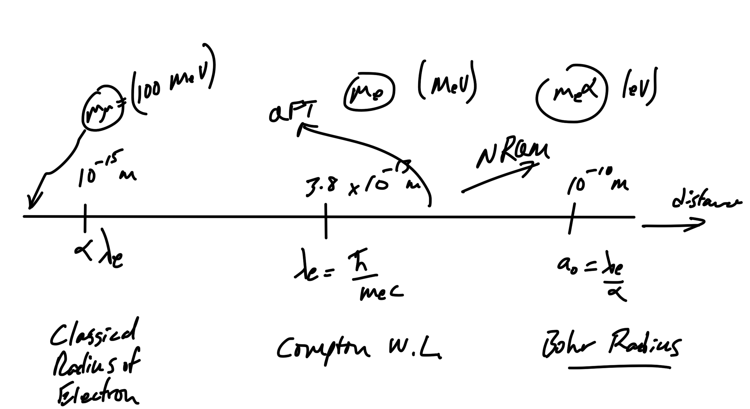
We can revisit the scale diagram from last lecture in terms of MeV mass/energy values, as sketched in fig. 1.

fig. 1. Scales, take II.

At the classical electron radius scale, we consider phenomena such as back reaction of radiation, the self energy of electrons. At the Compton wavelength we have to allow for production of multiple particle pairs. At Bohr radius scales we must start using QM instead of classical mechanics.

Cross section.

Verbal discussion of cross section, not captured in these notes. Roughly, the cross section sounds like the number of events per unit time, related to the flux of some source through an area.

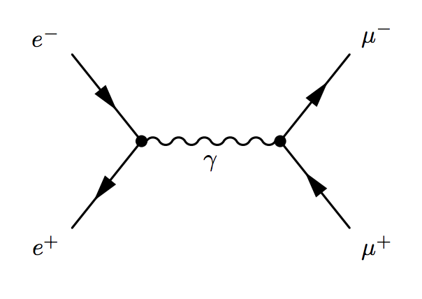
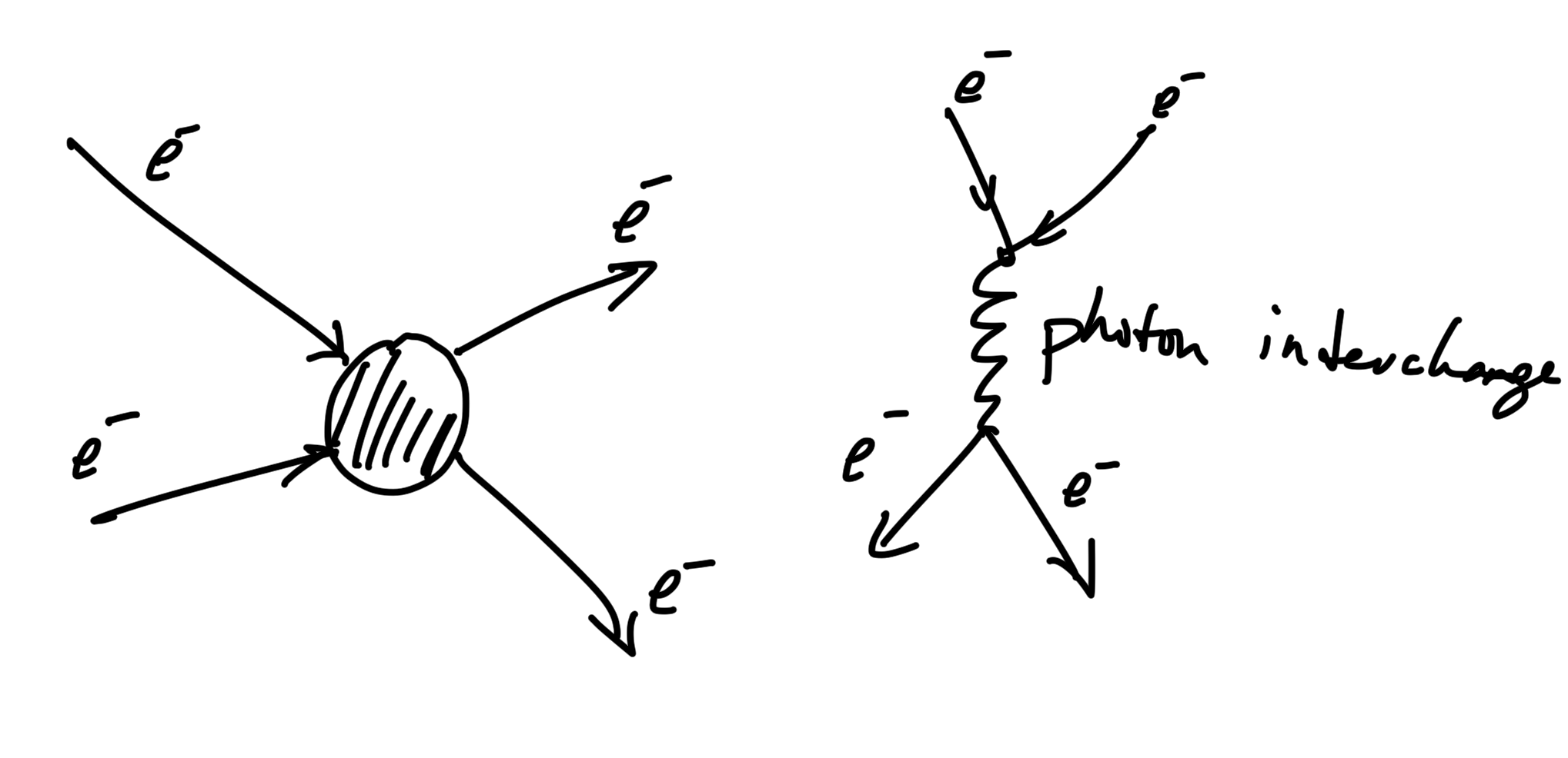
We’ll compute the cross section of a number of different systems in this course. The cross section is relevant in scattering such as the electron-electron scattering sketched in fig. 2.

fig. 2. Electron electron scattering.

We assume that QED is highly relativistic. In natural units, our scale factor is basically the square of the electric charge
\begin{equation}\label{eqn:qftLecture2:180}
\alpha \sim e^2,
\end{equation}
so the cross section has the form
\begin{equation}\label{eqn:qftLecture2:200}
\sigma \sim \frac{\alpha^2}{E^2} \lr{ 1 + O(\alpha) + O(\alpha^2) + \cdots }
\end{equation}

In gravity we could consider scattering of electrons, where \( G_\txtN \) takes the place of \( \alpha \). However, \( G_\txtN \) has dimensions.

For electron-electron scattering due to gravitons

\begin{equation}\label{eqn:qftLecture2:220}
\sigma \sim \frac{G_\txtN^2 E^2}{1 + G_\txtN E^2 + \cdots }
\end{equation}

Now the cross section grows with energy. This will cause some problems (violating unitarity: probabilities greater than 1!) when \( O(G_\txtN E^2) = 1 \).

In any quantum field theories when the coupling constant is not-dimensionless we have the same sort of problems at some scale.

The point is that we can get far considering just dimensional analysis.

If the coupling constant has a dimension \((1/\text{mass})^N\,, N > 0\), then unitarity will be violated at high energy. One such theory is the Fermi theory of beta decay (electro-weak theory), which had a coupling constant with dimensions inverse-mass-squared. The relevant scale for beta decay was 4 Fermi, or \( G_\txtF \sim (1/{100 \text{GeV}})^2 \). This was the motivation for introducing the Higgs theory, which was motivated by restoring unitarity.

Lorentz transformations.

The goal, perhaps not for today, is to study the simplest (relativistic) scalar field theory. First studied classically, and then consider such a quantum field theory.

How is relativity implemented when we write the Lagrangian and action?

Our first step must be to consider Lorentz transformations and the Lorentz group.

Spacetime (Minkowski space) is \R{3,1} (or \R{d-1,1}). Our coordinates are

\begin{equation}\label{eqn:qftLecture2:340}
(c t, x^1, x^2, x^3) = (c t, \Br).
\end{equation}

Here, we’ve scaled the time scale by \( c \) so that we measure time and space in the same dimensions. We write this as

\begin{equation}\label{eqn:qftLecture2:360}
x^\mu = (x^0, x^1, x^2, x^3),
\end{equation}

where \( \mu = 0, 1, 2, 3 \), and call this a “4-vector”. These are called the space-time coordinates of an event, which tell us where and when an event occurs.

For two events whose spacetime coordinates differ by \( dx^0, dx^1, dx^2, dx^3 \) we introduce the notion of a space time \underline{interval}

\begin{equation}\label{eqn:qftLecture2:380}
\begin{aligned}
ds^2
&= c^2 dt^2
– (dx^1)^2
– (dx^2)^2
– (dx^3)^2 \\
&=
\sum_{\mu, \nu = 0}^3 g_{\mu\nu} dx^\mu dx^\nu
\end{aligned}
\end{equation}

Here \( g_{\mu\nu} \) is the Minkowski space metric, an object with two indexes that run from 0-3. i.e. this is a diagonal matrix

\begin{equation}\label{eqn:qftLecture2:400}
g_{\mu\nu} \sim
\begin{bmatrix}
1 & 0 & 0 & 0 \\
0 & -1 & 0 & 0 \\
0 & 0 & -1 & 0 \\
0 & 0 & 0 & -1 \\
\end{bmatrix}
\end{equation}

i.e.
\begin{equation}\label{eqn:qftLecture2:420}
\begin{aligned}
g_{00} &= 1 \\
g_{11} &= -1 \\
g_{22} &= -1 \\
g_{33} &= -1 \\
\end{aligned}
\end{equation}

We will use the Einstein summation convention, where any repeated upper and lower indexes are considered summed over. That is \ref{eqn:qftLecture2:380} is written with an implied sum
\begin{equation}\label{eqn:qftLecture2:440}
ds^2 = g_{\mu\nu} dx^\mu dx^\nu.
\end{equation}

Explicit expansion:
\begin{equation}\label{eqn:qftLecture2:460}
\begin{aligned}
ds^2
&= g_{\mu\nu} dx^\mu dx^\nu \\
&=
g_{00} dx^0 dx^0
+g_{11} dx^1 dx^1
+g_{22} dx^2 dx^2
+g_{33} dx^3 dx^3
&=
(1) dx^0 dx^0
+ (-1) dx^1 dx^1
+ (-1) dx^2 dx^2
+ (-1) dx^3 dx^3.
\end{aligned}
\end{equation}

Recall that rotations (with orthogonal matrix representations) are transformations that leave the dot product unchanged, that is

\begin{equation}\label{eqn:qftLecture2:480}
\begin{aligned}
(R \Bx) \cdot (R \By)
&= \Bx^\T R^\T R \By \\
&= \Bx^\T \By \\
&= \Bx \cdot \By,
\end{aligned}
\end{equation}

where \( R \) is a rotation orthogonal 3×3 matrix. The set of such transformations that leave the dot product unchanged have orthonormal matrix representations \( R^\T R = 1 \). We call the set of such transformations that have unit determinant the SO(3) group.

We call a Lorentz transformation, if it is a linear transformation acting on 4 vectors that leaves the spacetime interval (i.e. the inner product of 4 vectors) invariant. That is, a transformation that leaves
\begin{equation}\label{eqn:qftLecture2:500}
x^\mu y^\nu g_{\mu\nu} = x^0 y^0 – x^1 y^1 – x^2 y^2 – x^3 y^3
\end{equation}
unchanged.

Suppose that transformation has a 4×4 matrix form

\begin{equation}\label{eqn:qftLecture2:520}
{x’}^\mu = {\Lambda^\mu}_\nu x^\nu
\end{equation}

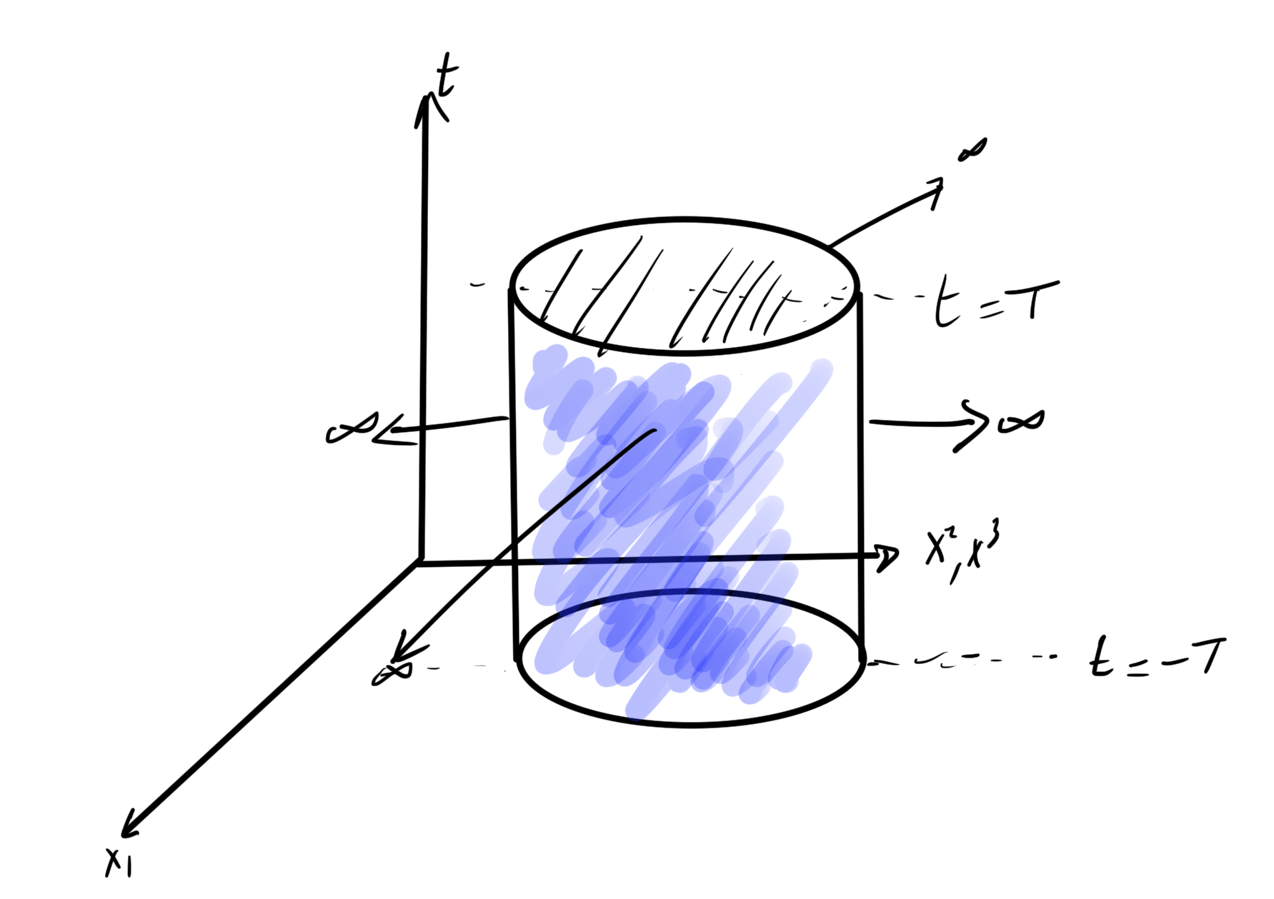
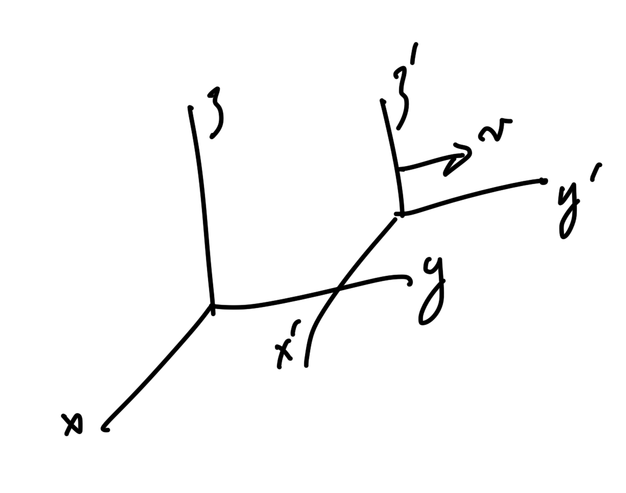
For an example of a possible \( \Lambda \), consider the transformation sketched in fig. 3.

fig. 3. Boost transformation.

We know that boost has the form
\begin{equation}\label{eqn:qftLecture2:540}
\begin{aligned}
x &= \frac{x’ + v t’}{\sqrt{1 – v^2/c^2}} \\
y &= y’ \\
z &= z’ \\
t &= \frac{t’ + (v/c^2) x’}{\sqrt{1 – v^2/c^2}} \\
\end{aligned}
\end{equation}
(this is a boost along the x-axis, not y as I’d drawn),
or
\begin{equation}\label{eqn:qftLecture2:560}
\begin{bmatrix}
c t \\
x \\
y \\
z
\end{bmatrix}
=
\begin{bmatrix}
\inv{\sqrt{1 – v^2/c^2}} & \frac{v/c}{\sqrt{1 – v^2/c^2}} & 0 & 0 \\
\frac{v/c}{\sqrt{1 – v^2/c^2}} & \frac{1}{\sqrt{1 – v^2/c^2}} & 0 & 0 \\
0 & 0 & 1 & 0 \\
0 & 0 & 0 & 1 \\
\end{bmatrix}
\begin{bmatrix}
c t’ \\
x’ \\
y’ \\
z’
\end{bmatrix}
\end{equation}

Other examples include rotations (\({\lambda^0}_0 = 1\) zeros in \( {\lambda^0}_k, {\lambda^k}_0 \), and a rotation matrix in the remainder.)

Back to Lorentz transformations (\(\text{SO}(1,3)^+\)), let
\begin{equation}\label{eqn:qftLecture2:600}
\begin{aligned}
{x’}^\mu &= {\Lambda^\mu}_\nu x^\nu \\
{y’}^\kappa &= {\Lambda^\kappa}_\rho y^\rho
\end{aligned}
\end{equation}

The dot product
\begin{equation}\label{eqn:qftLecture2:620}
g_{\mu \kappa}
{x’}^\mu
{y’}^\kappa
=
g_{\mu \kappa}
{\Lambda^\mu}_\nu
{\Lambda^\kappa}_\rho
x^\nu
y^\rho
=
g_{\nu\rho}
x^\nu
y^\rho,
\end{equation}
where the last step introduces the invariance requirement of the transformation. That is

\begin{equation}\label{eqn:qftLecture2:640}
\boxed{
g_{\nu\rho}
=
g_{\mu \kappa}
{\Lambda^\mu}_\nu
{\Lambda^\kappa}_\rho.
}
\end{equation}

Upper and lower indexes

We’ve defined

\begin{equation}\label{eqn:qftLecture2:660}
x^\mu = (t, x^1, x^2, x^3)
\end{equation}

We could also define a four vector with lower indexes
\begin{equation}\label{eqn:qftLecture2:680}
x_\nu = g_{\nu\mu} x^\mu = (t, -x^1, -x^2, -x^3).
\end{equation}
That is
\begin{equation}\label{eqn:qftLecture2:700}
\begin{aligned}
x_0 &= x^0 \\
x_1 &= -x^1 \\
x_2 &= -x^2 \\
x_3 &= -x^3.
\end{aligned}
\end{equation}

which allows us to write the dot product as simply \( x^\mu y_\mu \).

We can also define a metric tensor with upper indexes

\begin{equation}\label{eqn:qftLecture2:401}
g^{\mu\nu} \sim
\begin{bmatrix}
1 & 0 & 0 & 0 \\
0 & -1 & 0 & 0 \\
0 & 0 & -1 & 0 \\
0 & 0 & 0 & -1 \\
\end{bmatrix}
\end{equation}
This is the inverse matrix of \( g_{\mu\nu} \), and it satisfies
\begin{equation}\label{eqn:qftLecture2:720}
g^{\mu \nu} g_{\nu\rho} = {\delta^\mu}_\rho
\end{equation}

Exercise: Check:
\begin{equation}\label{eqn:qftLecture2:740}
\begin{aligned}
g_{\mu\nu} x^\mu y^\nu
&= x_\nu y^\nu \\
&= x^\nu y_\nu \\
&= g^{\mu\nu} x_\mu y_\nu \\
&= {\delta^\mu}_\nu x_\mu y^\nu.
\end{aligned}
\end{equation}

Class ended around this point, but it appeared that we were heading this direction:

Returning to the Lorentz invariant and multiplying both sides of
\ref{eqn:qftLecture2:640} with an inverse Lorentz transformation \( \Lambda^{-1} \), we find
\begin{equation}\label{eqn:qftLecture2:760}
\begin{aligned}
g_{\nu\rho}
{\lr{\Lambda^{-1}}^\rho}_\alpha
&=
g_{\mu \kappa}
{\Lambda^\mu}_\nu
{\Lambda^\kappa}_\rho
{\lr{\Lambda^{-1}}^\rho}_\alpha \\
&=
g_{\mu \kappa}
{\Lambda^\mu}_\nu
{\delta^\kappa}_\alpha \\
&=
g_{\mu \alpha}
{\Lambda^\mu}_\nu,
\end{aligned}
\end{equation}
or
\begin{equation}\label{eqn:qftLecture2:780}
\lr{\Lambda^{-1}}_{\nu \alpha} = \Lambda_{\alpha \nu}.
\end{equation}
This is clearly analogous to \( R^\T = R^{-1} \), although the index notation obscures things considerably. Prof. Poppitz said that next week this would all lead to showing that the determinant of any Lorentz transformation was \( \pm 1 \).

For what it’s worth, it seems to me that this index notation makes life a lot harder than it needs to be, at least for a matrix related question (i.e. determinant of the transformation). In matrix/column-(4)-vector notation, let \(x’ = \Lambda x, y’ = \Lambda y\) be two four vector transformations, then
\begin{equation}\label{eqn:qftLecture2:800}
x’ \cdot y’ = {x’}^T G y’ = (\Lambda x)^T G \Lambda y = x^T ( \Lambda^T G \Lambda) y = x^T G y.
\end{equation}
so
\begin{equation}\label{eqn:qftLecture2:820}
\boxed{
\Lambda^T G \Lambda = G.
}
\end{equation}
Taking determinants of both sides gives \(-(det(\Lambda))^2 = -1\), and thus \(det(\Lambda) = \pm 1\).

Awesome bookshelves in my home office space

September 15, 2018 Incoherent ramblings , ,

Sofia and I spend a large part of the day installing a set of four Ikea Liatorp bookshelves in my office today. The shelves fit pretty much perfectly, with a 1/4″ gap on each side. In fact, to get them to fit we had to take the baseboards and window casings off, but I’ll put in new ones butting up nicely to the shelves. When we eventually sell the house, the buyer better be interested in bookshelves, because these are a permanent feature of the house now!

The Liatorp model shelves are nicely engineered.  There are easy access leveling pegs, they join together nicely, and the backer board uses screws with pre-drilled holes in exactly the right places, plug some other plugs that hold the backer in place (far superior to the Billy model!)

Here’s a view of the whole shelf unit, which is loaded bottom heavy since the top shelves are spaces closer at the moment:

I had a lot of fun moving books down from the bedroom bookshelves, and have moved most of the non-fiction content.  I was really pleased that I can mostly group my books in logical categories:

  • Statistics and probability, with a couple German books and a dictionary too big to fit with the language material.
  • Calculus and engineering:

  • Computer programming, including my brand new Knuth box set!

  •  Spill over programming, general physics, fluid mechanics, and solid mechanics:

  • Home repair and handywork, plus two religious books too big to fit in the religion section (I’ve got other religious material in boxes somewhere in the basement, including a Morman bible, a Koran, and a whole lot of Dad’s Scientology books (and a couple of mine from days of old) :

  • Optics and statistical mechanics

  • Investment and economics (although the only one I’ve really cracked of these is the old “Principles of Engineering Economic Analysis” from back in my undergrad days)

  • Electromagnetism and some older general physics books from Granddad:

  • Algebra, complex variables, General relativity, mathematical tables, plus Penrose’s book, which spans most categories:

  • Political, classics, some borrowed Gaiman books, and religious

  • Languages:

There’s a bunch of tidy up and finishing details to make my office space complete and usable, but this was a really nice step in that direction.  Mysteriously, even after moving all these books downstairs from the bedroom, somehow the bedroom bookshelves are still mostly full seeming.  Was there a wild book orgy when we weren’t looking, and now all the book progeny are left behind, still filling the shelves despite the attempt to empty them?