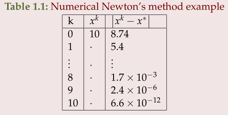
[Click here for a PDF of this post with nicer formatting]
Disclaimer
Peeter’s lecture notes from class. These may be incoherent and rough.
Fill ins
The problem of fill ins in LU computations arise in locations where rows and columns cross over zero positions.
Rows and columns can be permuted to deal with these. Here is an ad-hoc permutation of rows and columns that will result in less fill ins.
\begin{equation}\label{eqn:multiphysicsL7:180}
\begin{aligned}
&
\begin{bmatrix}
a & b & c & 0 \\
d & e & 0 & 0 \\
0 & f & g & 0 \\
0 & h & 0 & i \\
\end{bmatrix}
\begin{bmatrix}
x_1 \\
x_2 \\
x_3 \\
x_4
\end{bmatrix}
=
\begin{bmatrix}
b_1 \\
b_2 \\
b_3 \\
b_4
\end{bmatrix} \\
\Rightarrow &
\begin{bmatrix}
a & c & 0 & b \\
d & 0 & 0 & e \\
0 & g & 0 & f \\
0 & 0 & i & h \\
\end{bmatrix}
\begin{bmatrix}
x_1 \\
x_4 \\
x_3 \\
x_2 \\
\end{bmatrix}
=
\begin{bmatrix}
b_1 \\
b_2 \\
b_3 \\
b_4 \\
\end{bmatrix} \\
\Rightarrow &
\begin{bmatrix}
0 & a & c & b \\
0 & d & 0 & e \\
0 & 0 & g & f \\
i & 0 & 0 & h \\
\end{bmatrix}
\begin{bmatrix}
x_3 \\
x_4 \\
x_1 \\
x_2 \\
\end{bmatrix}
=
\begin{bmatrix}
b_1 \\
b_2 \\
b_3 \\
b_4 \\
\end{bmatrix} \\
\Rightarrow &
\begin{bmatrix}
i & 0 & 0 & h \\
0 & a & c & b \\
0 & d & 0 & e \\
0 & 0 & g & f \\
\end{bmatrix}
\begin{bmatrix}
x_3 \\
x_4 \\
x_1 \\
x_2 \\
\end{bmatrix}
=
\begin{bmatrix}
b_4 \\
b_1 \\
b_2 \\
b_3 \\
\end{bmatrix} \\
\Rightarrow &
\begin{bmatrix}
i & 0 & 0 & h \\
0 & c & a & b \\
0 & 0 & d & e \\
0 & g & 0 & f \\
\end{bmatrix}
\begin{bmatrix}
x_3 \\
x_1 \\
x_4 \\
x_2 \\
\end{bmatrix}
=
\begin{bmatrix}
b_4 \\
b_1 \\
b_2 \\
b_3 \\
\end{bmatrix} \\
\end{aligned}
\end{equation}
Markowitz product
To facilitate such permutations the Markowitz product that estimates the amount of fill in required.
Definition Markowitz product
\begin{equation*}
\begin{aligned}
\text{Markowitz product} =
&\lr{\text{Non zeros in unfactored part of Row -1}} \times \\
&\lr{\text{Non zeros in unfactored part of Col -1}}
\end{aligned}
\end{equation*}
In [1] it is stated “A still simpler alternative, which seems adequate generally, is to choose the pivot which minimizes the number of coefficients modified at each step (excluding those which are eliminated at the particular step). This is equivalent to choosing the non-zero element with minimum \( (\rho_i – 1 )(\sigma_j -1) \).”
Note that this product is applied only to \( i j \) positions that are
non-zero, something not explicitly mentioned in the slides, nor in other
locations like [2]
Example: Markowitz product
For this matrix
\begin{equation}\label{eqn:multiphysicsL7:220}
\begin{bmatrix}
a & b & c & 0 \\
d & e & 0 & 0 \\
0 & f & g & 0 \\
0 & h & 0 & i \\
\end{bmatrix},
\end{equation}
the Markowitz products are
\begin{equation}\label{eqn:multiphysicsL7:280}
\begin{bmatrix}
1 & 6 & 2 & \\
1 & 3 & & \\
& 3 & 1 & \\
& 3 & & 0 \\
\end{bmatrix}.
\end{equation}
Markowitz reordering
The Markowitz Reordering procedure (copied directly from the slides) is
- For i = 1 to n
- Find diagonal \( j >= i \) with min Markowitz product
- Swap rows \( j \leftrightarrow i \) and columns \( j \leftrightarrow i \)
- Factor the new row \( i \) and update Markowitz products
Example: Markowitz reordering
Looking at the Markowitz products \ref{eqn:multiphysicsL7:280} a swap of rows and columns \( 1, 4 \) gives the modified matrix
\begin{equation}\label{eqn:multiphysicsL7:300}
\begin{bmatrix}
i & 0 & h & 0 \\
0 & d & e & 0 \\
0 & 0 & f & g \\
0 & a & b & c \\
\end{bmatrix}
\end{equation}
In this case, this reordering has completely avoided any requirement to do any actual Gaussian operations for this first stage reduction.
Presuming that the Markowitz products for the remaining 3×3 submatrix are only computed from that submatrix, the new products are
\begin{equation}\label{eqn:multiphysicsL7:320}
\begin{bmatrix}
& & & \\
& 1 & 2 & \\
& & 2 & 1 \\
& 2 & 4 & 2 \\
\end{bmatrix}.
\end{equation}
We have a minimal product in the pivot position, which happens to already lie on the diagonal. Note that it is not necessarily the best for numerical stability. It appears the off diagonal Markowitz products are not really of interest since the reordering algorithm swaps both rows and columns.
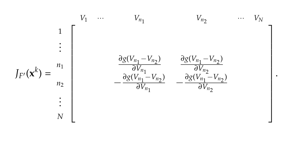
Graph representation
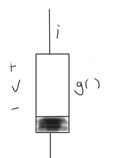
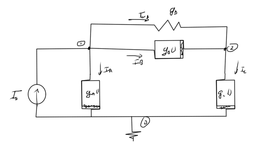
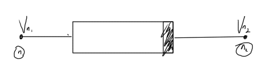
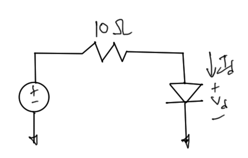
It is possible to interpret the Markowitz products on the diagonal as connectivity of a graph that represents the interconnections of the nodes. Consider the circuit of fig. 2 as an example
fig 2. Simple circuit
The system equations for this circuit is of the form
\begin{equation}\label{eqn:multiphysicsL7:340}
\begin{bmatrix}
x & x & x & 0 & 1 \\
x & x & x & 0 & 0 \\
x & x & x & x & 0 \\
0 & 0 & x & x & -1 \\
-1 & 0 & 0 & 1 & 0 \\
\end{bmatrix}
\begin{bmatrix}
V_1 \\
V_2 \\
V_3 \\
V_4 \\
i \\
\end{bmatrix}
=
\begin{bmatrix}
0 \\
0 \\
0 \\
0 \\
x \\
\end{bmatrix}.
\end{equation}
The Markowitz products along the diagonal are
\begin{equation}\label{eqn:multiphysicsL7:360}
\begin{aligned}
M_{11} &= 9 \\
M_{22} &= 4 \\
M_{33} &= 9 \\
M_{44} &= 4 \\
M_{55} &= 4 \\
\end{aligned}
\end{equation}
Compare these to the number of interconnections of the graph fig. 3 of the nodes in this circuit. We see that these are the squares of the number of the node interconnects in each case.
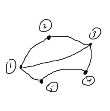
fig. 3. Graph representation
Here a 5th node was introduced for the current \( i \) between nodes \( 4 \) and \( 1 \). Observe that the Markowitz product of this node was counted as the number of non-zero values excluding the \( 5,5 \) matrix position. However, that doesn’t matter too much since a Markowitz swap of row/column 1 with row/column 5 would put a zero in the \( 1,1 \) position of the matrix, which is not desirable. We have to restrict the permutations of zero diagonal positions to pivots for numerical stability, or use a more advanced zero fill avoidance algorithm.
The minimum diagonal Markowitz products are in positions 2 or 4, with respective Markowitz reorderings of the form
\begin{equation}\label{eqn:multiphysicsL7:380}
\begin{bmatrix}
x & x & x & 0 & 0 \\
x & x & x & 0 & 1 \\
x & x & x & x & 0 \\
0 & 0 & x & x & -1 \\
0 & -1 & 0 & 1 & 0 \\
\end{bmatrix}
\begin{bmatrix}
V_2 \\
V_1 \\
V_3 \\
V_4 \\
i \\
\end{bmatrix}
=
\begin{bmatrix}
0 \\
0 \\
0 \\
0 \\
x \\
\end{bmatrix},
\end{equation}
and
\begin{equation}\label{eqn:multiphysicsL7:400}
\begin{bmatrix}
x & 0 & 0 & x & -1 \\
0 & x & x & x & 1 \\
0 & x & x & x & 0 \\
x & x & x & x & 0 \\
1 & -1 & 0 & 0 & 0 \\
\end{bmatrix}
\begin{bmatrix}
V_4 \\
V_1 \\
V_2 \\
V_3 \\
i \\
\end{bmatrix}
=
\begin{bmatrix}
0 \\
0 \\
0 \\
0 \\
x \\
\end{bmatrix}.
\end{equation}
The original system had 7 zeros that could potentially be filled in the remaining \( 4 \times 4 \) submatrix. After a first round of Gaussian elimination, our system matrices have the respective forms
\begin{equation}\label{eqn:multiphysicsL7:420}
\begin{bmatrix}
x & x & x & 0 & 0 \\
0 & x & x & 0 & 1 \\
0 & x & x & x & 0 \\
0 & 0 & x & x & -1 \\
0 & -1 & 0 & 1 & 0 \\
\end{bmatrix}
\end{equation}
\begin{equation}\label{eqn:multiphysicsL7:440}
\begin{bmatrix}
x & 0 & 0 & x & -1 \\
0 & x & x & x & 1 \\
0 & x & x & x & 0 \\
0 & x & x & x & 0 \\
0 & -1 & 0 & x & x \\
\end{bmatrix}
\end{equation}
The remaining \( 4 \times 4 \) submatrices have interconnect graphs sketched in fig. 4.
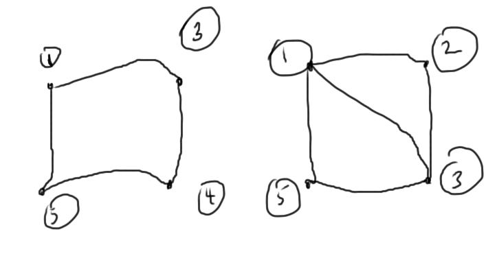
fig. 4. Graphs after one round of Gaussian elimination
From a graph point of view, we want to delete the most connected nodes. This can be driven by the Markowitz products along the diagonal or directly with graph methods.
Summary of factorization costs
LU (dense)
- cost: \( O(n^3) \)
- cost depends only on size
LU (sparse)
- cost: Diagonal and tridiagonal are \( O(n) \), but we can have up to \( O(n^3) \) depending on sparsity and the method of dealing with the sparsity.
- cost depends on size and sparsity
Computation can be affordable up to a few million elements.
Iterative methods
Can be cheap if done right. Convergence requires careful preconditioning.
Iterative methods
Suppose that we have an initial guess \( \Bx_0 \). Iterative methods are generally of the form
DO
\(\Br = \Bb – M \Bx_i\)
UNTIL \(\Norm{\Br} < \epsilon \)
The difference \( \Br \) is called the residual. For as long as it is bigger than desired, continue improving the estimate \( \Bx_i \).
The matrix vector product \( M \Bx_i \), if dense, is of \( O(n^2) \). Suppose, for example, that we can perform the iteration in ten iterations. If the matrix is dense, we can have \( 10 \, O(n^2) \) performance. If sparse, this can be worse than just direct computation.
Gradient method
This is a method for iterative solution of the equation \( M \Bx = \Bb \).
This requires symmetric positive definite matrix \( M = M^\T \), with \( M > 0 \).
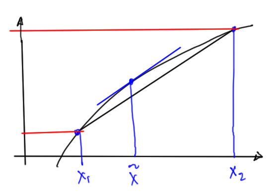
We introduce an energy function
\begin{equation}\label{eqn:multiphysicsL7:60}
\Psi(\By) \equiv \inv{2} \By^\T M \By – \By^\T \Bb
\end{equation}
For a two variable system this is illustrated in fig. 1.
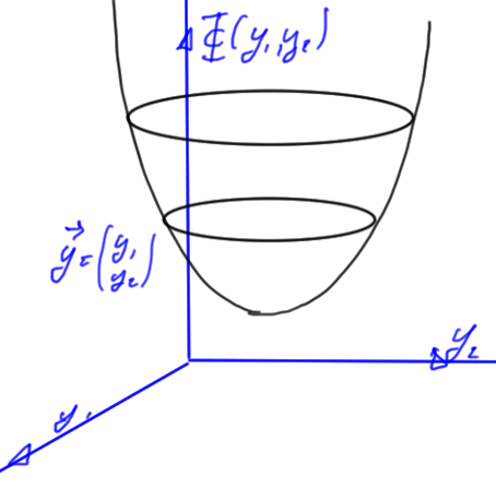
fig. 1. Positive definite energy function
Theorem: Energy function minimum
The energy function \ref{eqn:multiphysicsL7:60} has a minimum at
\begin{equation}\label{eqn:multiphysicsL7:80}
\By = M^{-1} \Bb = \Bx.
\end{equation}
To prove this, consider the coordinate representation
\begin{equation}\label{eqn:multiphysicsL7:480}
\Psi = \inv{2} y_a M_{ab} y_b – y_b b_b,
\end{equation}
for which the derivatives are
\begin{equation}\label{eqn:multiphysicsL7:500}
\PD{y_i}{\Psi} =
\inv{2} M_{ib} y_b
+
\inv{2} y_a M_{ai}
– b_i
=
\lr{ M \By – \Bb }_i.
\end{equation}
The last operation above was possible because \( M = M^\T \). Setting all of these equal to zero, and rewriting this as a matrix relation we have
\begin{equation}\label{eqn:multiphysicsL7:520}
M \By = \Bb,
\end{equation}
as asserted.
This is called the gradient method because the gradient moves us along the path of steepest descent towards the minimum if it exists.
The method is
\begin{equation}\label{eqn:multiphysicsL7:100}
\Bx^{(k+1)} = \Bx^{(k)} +
\underbrace{ \alpha_k }_{step size}
\underbrace{ \Bd^{(k)} }_{direction},
\end{equation}
where the direction is
\begin{equation}\label{eqn:multiphysicsL7:120}
\Bd^{(k)} = – \spacegrad \Phi = \Bb – M \Bx^k = r^{(k)}.
\end{equation}
Optimal step size
Note that for the minimization of \( \Phi \lr{ \Bx^{(k+1)} } \), we note
\begin{equation}\label{eqn:multiphysicsL7:140}
\Phi \lr{ \Bx^{(k+1)} }
= \Phi\lr{ \Bx^{(k)} + \alpha_k \Bd^{(k)} }
=
\inv{2}
\lr{ \Bx^{(k)} + \alpha_k \Bd^{(k)} }^\T
M
\lr{ \Bx^{(k)} + \alpha_k \Bd^{(k)} }
–
\lr{ \Bx^{(k)} + \alpha_k \Bd^{(k)} }^\T \Bb
\end{equation}
If we take the derivative of both sides with respect to \( \alpha_k \) to find the minimum, we have
\begin{equation}\label{eqn:multiphysicsL7:540}
0 =
\inv{2}
\lr{ \Bd^{(k)} }^\T
M
\Bx^{(k)}
+
\inv{2}
\lr{ \Bx^{(k)} }^\T
M
\Bd^{(k)}
+
\alpha_k \lr{ \Bd^{(k)} }^\T
M
\Bd^{(k)}
–
\lr{ \Bd^{(k)} }^\T \Bb.
\end{equation}
Because \( M \) is symmetric, this is
\begin{equation}\label{eqn:multiphysicsL7:560}
\alpha_k \lr{ \Bd^{(k)} }^\T
M
\Bd^{(k)}
=
\lr{ \Bd^{(k)} }^\T \lr{ \Bb – M \Bx^{(k)}}
=
\lr{ \Bd^{(k)} }^\T r^{(k)},
\end{equation}
or
\begin{equation}\label{eqn:multiphysicsL7:160}
\alpha_k
= \frac{
\lr{\Br^{(k)}}^\T
\Br^{(k)}
}{
\lr{\Br^{(k)}}^\T
M
\Br^{(k)}
}
\end{equation}
We will see that this method is not optimal when we pick one direction and keep going down that path.
Definitions and theorems
Definition: Positive (negative) definite
A matrix \( M \) is positive (negative) definite, denoted \( M > 0 (<0) \) if \( \By^\T M \By > 0 (<0), \quad \forall \By \).
If a matrix is neither positive, nor negative definite, it is called indefinite.
Theorem: Positive (negative) definite
A symmetric matrix \( M > 0 (<0)\) iff \( \lambda_i > 0 (<0)\) for all eigenvalues \( \lambda_i \), or is indefinite iff its eigenvalues \( \lambda_i \) are of mixed sign.
References
[1] Harry M Markowitz. The elimination form of the inverse and its application to linear programming. Management Science, 3\penalty0 (3):\penalty0 255–269, 1957.
[2] Timothy Vismor. Pivoting To Preserve Sparsity, 2012. URL https://vismor.com/documents/network_analysis/matrix_algorithms/S8.SS3.php. [Online; accessed 15-Oct-2014].