[Click here for a PDF of this post with nicer formatting]
Disclaimer
Peeter’s lecture notes from class. These may be incoherent and rough.
These are notes for the UofT course PHY1520, Graduate Quantum Mechanics, taught by Prof. Paramekanti, covering [1] chap. 2 content.
problem set note.
In the problem set we’ll look at interference patterns for two slit electron interference like that of fig. 1, where a magnetic whisker that introduces flux is added to the configuration.
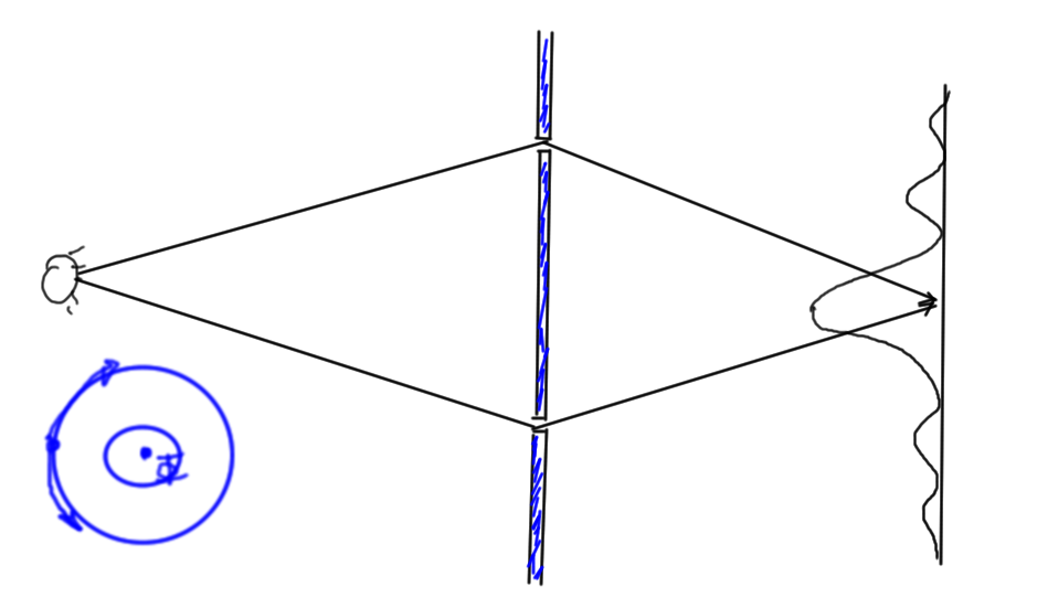
fig. 1. Two slit interference with magnetic whisker
Aharonov-Bohm effect (cont.)
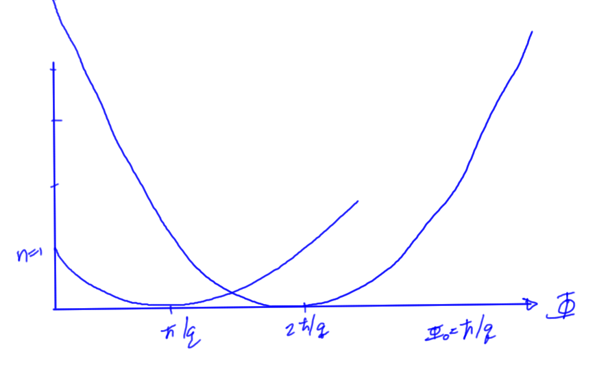
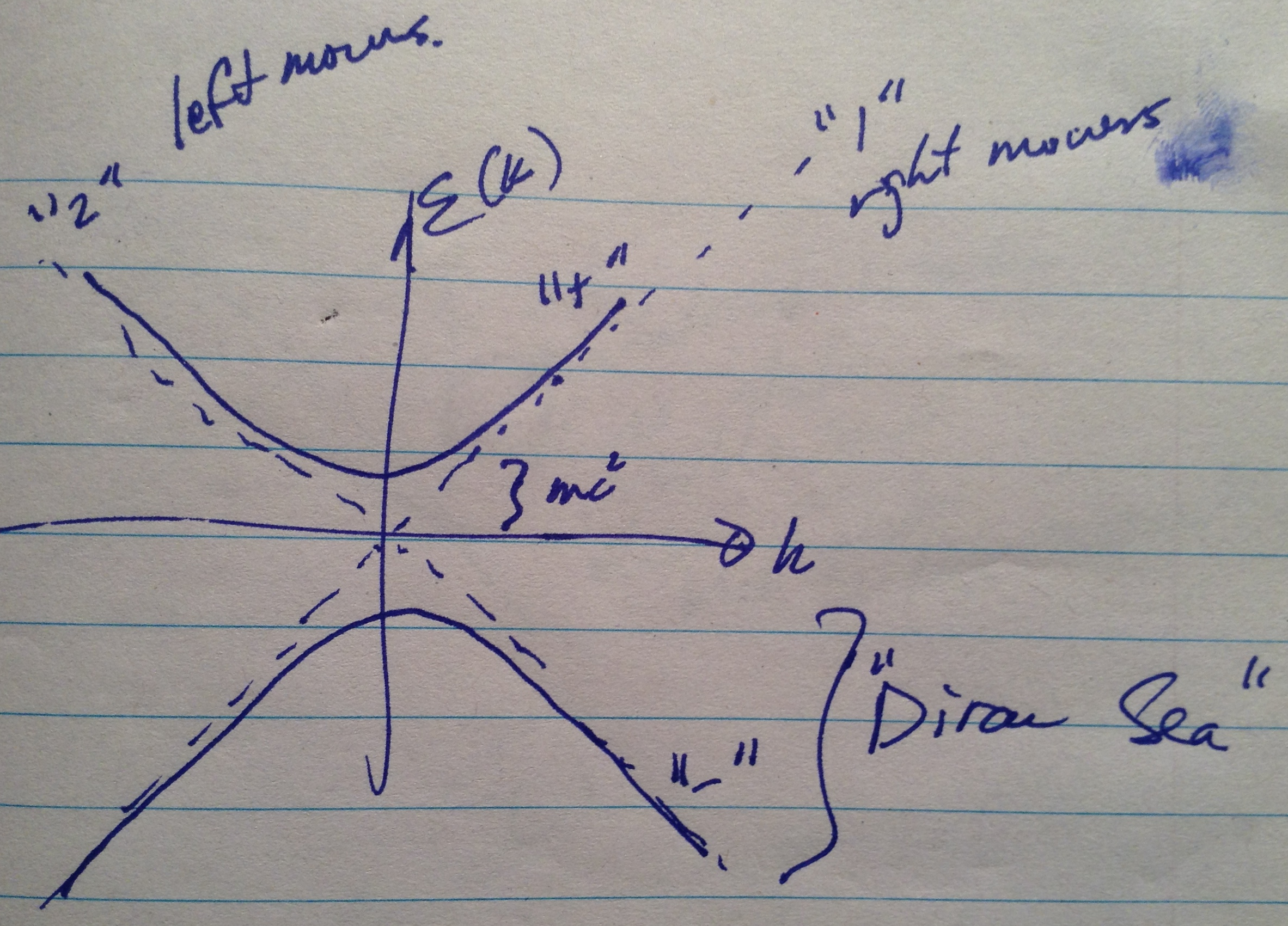
fig. 2. Energy vs flux
Why do we have the zeros at integral multiples of \( h/q \)? Consider a particle in a circular trajectory as sketched in fig. 3
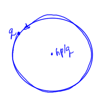
fig. 3. Circular trajectory
FIXME: Prof mentioned:
\begin{equation}\label{eqn:qmLecture7:20}
\phi_{\textrm{loop}} = q \frac{ h p/ q }{\Hbar} = 2 \pi p
\end{equation}
… I’m not sure what that was about now.
In classical mechanics we have
\begin{equation}\label{eqn:qmLecture7:40}
\oint p dq
\end{equation}
The integral zero points are related to such a loop, but the \( q \BA \) portion of the momentum \( \Bp – q \BA \) needs to be considered.
Superconductors
After cooling some materials sufficiently, superconductivity, a complete lack of resistance to electrical flow can be observed. A resistivity vs temperature plot of such a material is sketched in fig. 4.
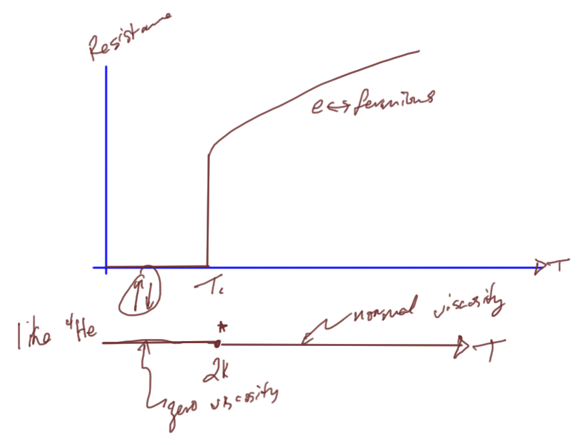
fig. 4. Superconductivity with comparison to superfluidity
Just like \ce{He^4} can undergo Bose condensation, superconductivity can be explained by a hybrid Bosonic state where electrons are paired into one state containing integral spin.
The Little-Parks experiment puts a superconducting ring around a magnetic whisker as sketched in fig. 6.
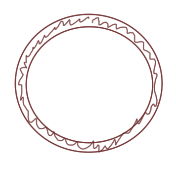
fig. 6. Little-Parks superconducting ring
This experiment shows that the effective charge of the circulating charge was \( 2 e \), validating the concept of Cooper-pairing, the Bosonic combination (integral spin) of electrons in superconduction.
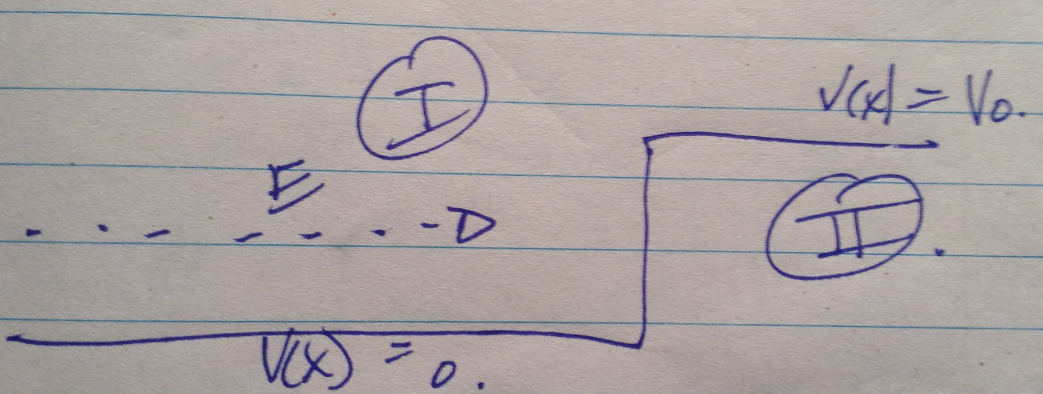
Motion around magnetic field
\begin{equation}\label{eqn:qmLecture7:140}
\omega_{\textrm{c}} = \frac{e B}{m}
\end{equation}
We work with what is now called the Landau gauge
\begin{equation}\label{eqn:qmLecture7:60}
\BA = \lr{ 0, B x, 0 }
\end{equation}
This gives
\begin{equation}\label{eqn:qmLecture7:80}
\begin{aligned}
\BB
&= \spacegrad \cross \BA \\
&= \lr{ \partial_x A_y – \partial_y A_x } \zcap \\
&= B \zcap.
\end{aligned}
\end{equation}
An alternate gauge choice, the symmetric gauge, is
\begin{equation}\label{eqn:qmLecture7:100}
\BA = \lr{ -\frac{B y}{2}, \frac{B x}{2}, 0 },
\end{equation}
that also has the same magnetic field
\begin{equation}\label{eqn:qmLecture7:120}
\begin{aligned}
\BB
&= \spacegrad \BA \\
&= \lr{ \partial_x A_y – \partial_y A_x } \zcap \\
&= \lr{ \frac{B}{2} – \lr{ – \frac{B}{2} } } \zcap \\
&= B \zcap.
\end{aligned}
\end{equation}
We expect the physics for each to have the same results, although the wave functions in one gauge may be more complicated than in the other.
Our Hamiltonian is
\begin{equation}\label{eqn:qmLecture7:160}
\begin{aligned}
H
&= \inv{2 m} \lr{ \Bp – e \BA }^2 \\
&= \inv{2 m} \hat{p}_x^2 + \inv{2 m} \lr{ \hat{p}_y – e B \xhat }^2
\end{aligned}
\end{equation}
We can solve after noting that
\begin{equation}\label{eqn:qmLecture7:180}
\antisymmetric{\hat{p}_y}{H} = 0
\end{equation}
means that
\begin{equation}\label{eqn:qmLecture7:200}
\Psi(x,y) = e^{i k_y y} \phi(x)
\end{equation}
The eigensystem
\begin{equation}\label{eqn:qmLecture7:220}
H \psi(x, y) = E \phi(x, y) ,
\end{equation}
becomes
\begin{equation}\label{eqn:qmLecture7:240}
\lr{ \inv{2 m} \hat{p}_x^2 + \inv{2 m} \lr{ \Hbar k_y – e B \xhat}^2 } \phi(x)
= E \phi(x).
\end{equation}
This reduced Hamiltonian can be rewritten as
\begin{equation}\label{eqn:qmLecture7:320}
H_x
= \inv{2 m} p_x^2 + \inv{2 m} e^2 B^2 \lr{ \xhat – \frac{\Hbar k_y}{e B} }^2
\equiv \inv{2 m} p_x^2 + \inv{2} m \omega^2 \lr{ \xhat – x_0 }^2
\end{equation}
where
\begin{equation}\label{eqn:qmLecture7:260}
\inv{2 m} e^2 B^2 = \inv{2} m \omega^2,
\end{equation}
or
\begin{equation}\label{eqn:qmLecture7:280}
\omega = \frac{ e B}{m} \equiv \omega_{\textrm{c}}.
\end{equation}
and
\begin{equation}\label{eqn:qmLecture7:300}
x_0 = \frac{\Hbar}{k_y}{e B}.
\end{equation}
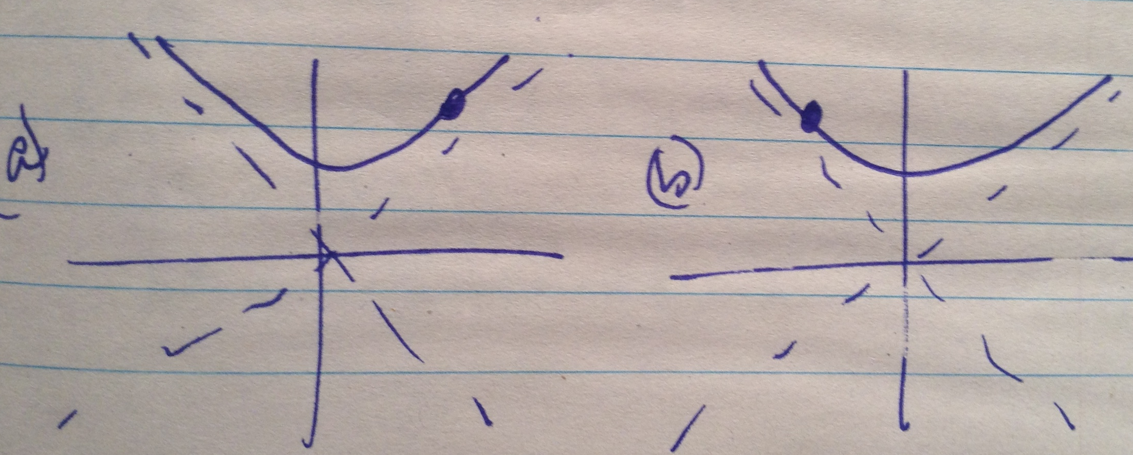
But what is this \( x_0 \)? Because \( k_y \) is not really specified in this problem, we can consider that we have a zero point energy for every \( k_y \), but the oscillator position is shifted for every such value of \( k_y \). For each set of energy levels fig. 8 we can consider that there is a different zero point energy for each possible \( k_y \).
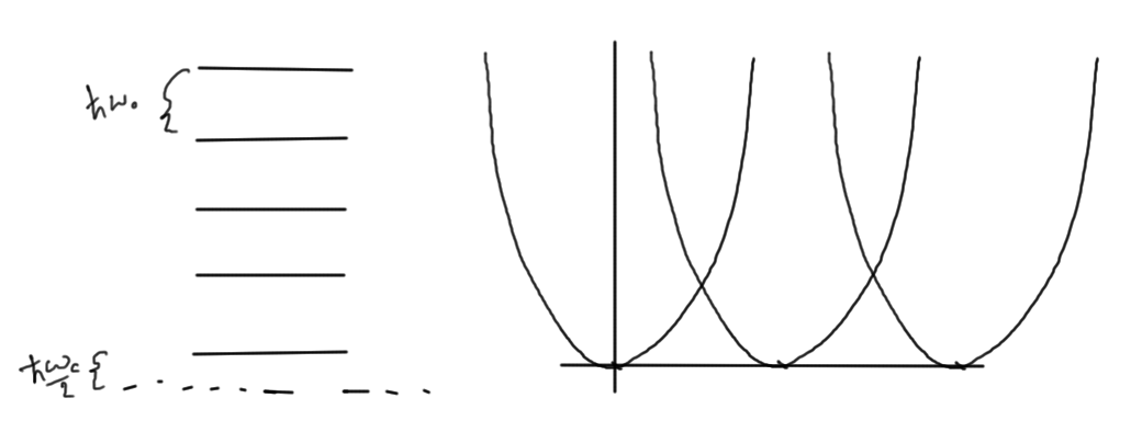
fig. 8. Energy levels, and Energy vs flux
This is an infinitely degenerate system with an infinite number of states for any given energy level.
This tells us that there is a problem, and have to reconsider the assumption that any \( k_y \) is acceptable.
To resolve this we can introduce periodic boundary conditions, imagining that a square is rotated in space forming a cylinder as sketched in fig. 9.
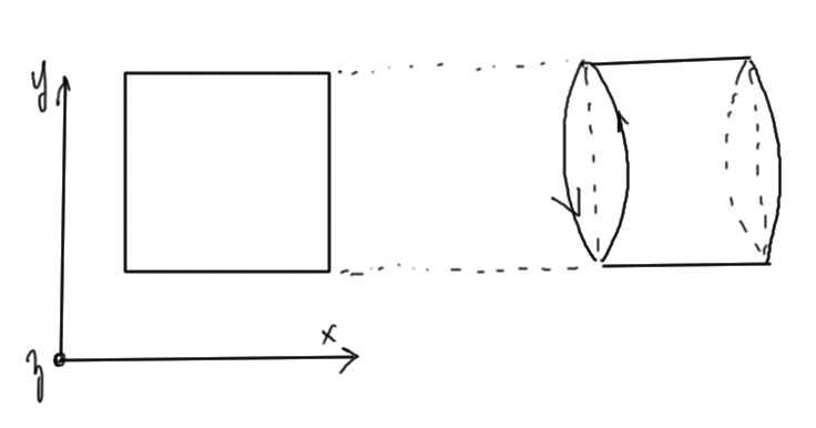
fig. 9. Landau degeneracy region
Requiring quantized momentum
\begin{equation}\label{eqn:qmLecture7:340}
k_y L_y = 2 \pi n,
\end{equation}
or
\begin{equation}\label{eqn:qmLecture7:360}
k_y = \frac{2 \pi n}{L_y}, \qquad n \in \mathbb{Z},
\end{equation}
gives
\begin{equation}\label{eqn:qmLecture7:380}
x_0(n) = \frac{\Hbar}{e B} \frac{ 2 \pi n}{L_y},
\end{equation}
with \( x_0 \le L_x \). The range is thus restricted to
\begin{equation}\label{eqn:qmLecture7:400}
\frac{\Hbar}{e B} \frac{ 2 \pi n_{\textrm{max}}}{L_y} = L_x,
\end{equation}
or
\begin{equation}\label{eqn:qmLecture7:420}
n_{\textrm{max}} = \underbrace{L_x L_y}_{\text{area}} \frac{ e B }{2 \pi \Hbar }
\end{equation}
That is
\begin{equation}\label{eqn:qmLecture7:440}
\begin{aligned}
n_{\textrm{max}}
&= \frac{\Phi_{\textrm{total}}}{h/e} \\
&= \frac{\Phi_{\textrm{total}}}{\Phi_0}.
\end{aligned}
\end{equation}
Attempting to measure Hall-effect systems, it was found that the Hall conductivity was quantized like
\begin{equation}\label{eqn:qmLecture7:460}
\sigma_{x y} = p \frac{e^2}{h}.
\end{equation}
This quantization is explained by these Landau levels, and this experimental apparatus provides one of the more accurate ways to measure the fine structure constant.
References
[1] Jun John Sakurai and Jim J Napolitano. Modern quantum mechanics. Pearson Higher Ed, 2014.