[Click here for a PDF of this post with nicer formatting]
Disclaimer
Peeter’s lecture notes from class. These may be incoherent and rough.
These are notes for the UofT course PHY1520, Graduate Quantum Mechanics, taught by Prof. Paramekanti, covering [1] chap. 3 content.
Clebsch-Gordan
How can we related total momentum states to individual momentum states in the \( 1 \otimes 2 \) space?
\begin{equation}\label{eqn:qmLecture16:720}
\ket{l_1, l_2, l, m } = \sum_{m_1, m_2} C_{l_1 l_2 m_1 m_2}^{l_1 l_2 l m} \ket{l_1 m_1 ; l_2 m_2 }
\end{equation}
The values \( C_{l_1 l_2 m_1 m_2}^{l_1 l_2 l m} \) are called the Clebsch-Gordan coefficients.
Example: spin one and spin one half
With individual momentum states \( \ket{l_1 m_1 ; l_2 m_2 } \)
\begin{equation}\label{eqn:qmLecture16:740}
\begin{aligned}
l_1 &= 1 \\
m_1 &= \pm 1, 0 \\
l_2 &= \inv{2} \\
m_2 &= \pm \inv{2}
\end{aligned}
\end{equation}
The total angular momentum numbers are
\begin{equation}\label{eqn:qmLecture16:760}
l_{\textrm{tot}} \in [l_1 – l_2, l_1 + l_2] = [\ifrac{1}{2}, \ifrac{3}{2}]
\end{equation}
The possible states \( \ket{ l_{\textrm{tot}}, m_{\textrm{tot}} } \) are
\begin{equation}\label{eqn:qmLecture16:780}
\ket{\inv{2}, \inv{2} }, \ket{\inv{2}, -\inv{2} },
\end{equation}
and
\begin{equation}\label{eqn:qmLecture16:800}
\ket{\frac{3}{2}, \frac{3}{2} }, \ket{\frac{3}{2}, \frac{1}{2} },
\ket{\frac{3}{2}, -\frac{1}{2} }
\ket{\frac{3}{2}, -\frac{3}{2} }.
\end{equation}
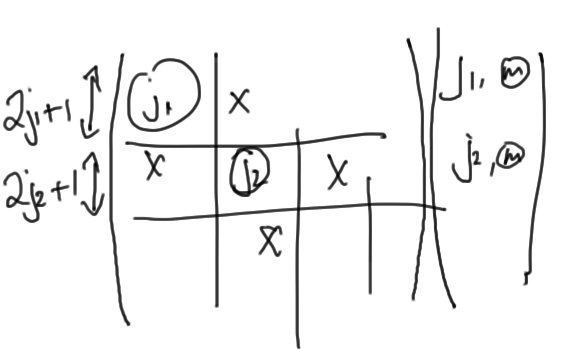
The Clebsch-Gordan procedure is the search for an orthogonal angular momentum basis, built up from the individual momentum bases. For the total momentum basis we want the basis states to satisfy the ladder operators, but also have them satisfy the consistuient ladder operators for the individual particle angular momenta. This procedure is sketched in fig. 1.
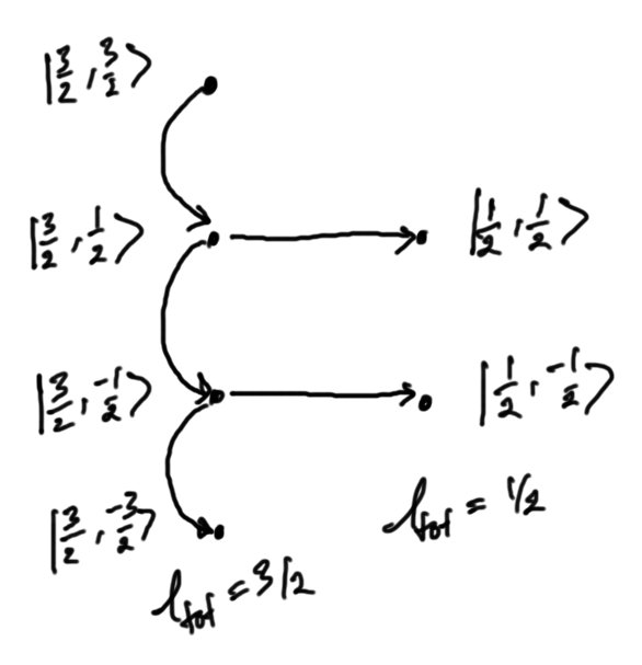
fig. 1. Spin one,one-half Clebsch-Gordan procedure
Demonstrating by example, let the highest total momentum state be proportional to the highest product of individual momentum states
\begin{equation}\label{eqn:qmLecture16:820}
\ket{ \frac{3}{2} \frac{3}{2} } = \ket{ 1 1 } \otimes \ket{ \frac{1}{2} \frac{1}{2} }.
\end{equation}
A lowered state can be constructed in two different ways, one using the total angular momentum lowering operator
\begin{equation}\label{eqn:qmLecture16:840}
\begin{aligned}
\ket{ \frac{3}{2} \frac{1}{2} }
&=
\hat{L}_{-}^{\textrm{tot}} \ket{ \frac{3}{2} \frac{3}{2} } \\
&= \Hbar \sqrt{\lr{\frac{3}{2} + \frac{3}{2}}\lr{\frac{3}{2} – \frac{3}{2} + 1}} \ket{ \frac{3}{2} \frac{1}{2} } \\
&= \Hbar \sqrt{3} \ket{ \frac{3}{2} \frac{1}{2} }.
\end{aligned}
\end{equation}
On the other hand, the lowering operator can also be expressed as \( \hat{L}_{-}^{\textrm{tot}} = \hat{L}_{-}^{(1)} \otimes 1 + 1 \otimes \hat{L}_{-}^{(2)} \). Operating with that gives
\begin{equation}\label{eqn:qmLecture16:860}
\begin{aligned}
\ket{ \frac{3}{2} \frac{1}{2} }
&=
\hat{L}_{-}^{\textrm{tot}} \ket{ 1 1 } \otimes \ket{ \frac{1}{2} \frac{1}{2} }
\\
&=
\hat{L}_{-}^{(1)} \ket{ 1 1 } \otimes \ket{ \frac{1}{2} \frac{1}{2} }
+
\ket{ 1 1 } \otimes \hat{L}_{-}^2 \ket{ \frac{1}{2} \frac{1}{2} } \\
&=
\Hbar \sqrt{\lr{1 + 1}\lr{1 – 1 + 1}} \ket{ 1 0 } \otimes \ket{ \frac{1}{2} \frac{1}{2} }
+
\Hbar \sqrt{\lr{\frac{1}{2} + \frac{1}{2}}\lr{\frac{1}{2} – \frac{1}{2} + 1}}
\ket{ 1 1 } \otimes \ket{ \frac{1}{2} -\frac{1}{2} } \\
&=
\Hbar \sqrt{2} \ket{ 1 0 } \otimes \ket{ \frac{1}{2} \frac{1}{2} }
+
\Hbar \ket{ 1 1 } \otimes \ket{ \frac{1}{2} -\frac{1}{2} }.
\end{aligned}
\end{equation}
Equating both sides and dispensing with the direct product notation, this is
\begin{equation}\label{eqn:qmLecture16:880}
\sqrt{3} \ket{ \frac{3}{2} \frac{1}{2} }
=
\sqrt{2} \ket{ 1 0 ; \frac{1}{2} \frac{1}{2} }
+
\ket{ 1 1 ; \frac{1}{2} -\frac{1}{2} },
\end{equation}
or
\begin{equation}\label{eqn:qmLecture16:900}
\boxed{
\ket{ \frac{3}{2} \frac{1}{2} }
=
\sqrt{\frac{2}{3}} \ket{ 1 0 ; \frac{1}{2} \frac{1}{2} }
+
\inv{\sqrt{3}} \ket{ 1 1 ; \frac{1}{2} -\frac{1}{2} }.
}
\end{equation}
This is clearly both a unit ket, and normal to \( \ket{ \frac{3}{2} \frac{3}{2} } \). We can continue operating with the lowering operator for the total angular momentum to constuct all the states down to \( \ket{ \frac{3}{2} \frac{-3}{2} } \). Working with \( \Hbar = 1 \) since we see it cancel out, the next lower state follows from
\begin{equation}\label{eqn:qmLecture16:920}
\begin{aligned}
\hat{L}_{-}^{\textrm{tot}} \ket{ \frac{3}{2} \frac{1}{2} }
&=
\sqrt{2 \times 2} \ket{ \frac{3}{2} \frac{-1}{2} } \\
&=
2 \ket{ \frac{3}{2} \frac{-1}{2} }.
\end{aligned}
\end{equation}
and from the individual lowering operators on the components of \( \ket{ \frac{3}{2} \frac{1}{2} } \).
\begin{equation}\label{eqn:qmLecture16:940}
\hat{L}_{-}^{(1)} \ket{ 1 0 ; \frac{1}{2} \frac{1}{2} }
=
\sqrt{ 1 \times 2 } \ket{ 1 -1 ; \frac{1}{2} \frac{1}{2} },
\end{equation}
and
\begin{equation}\label{eqn:qmLecture16:960}
\hat{L}_{-}^{(2)} \ket{ 1 0 ; \frac{1}{2} \frac{1}{2} }
=
\sqrt{ 1 \times 1 } \ket{ 1 0 ; \frac{1}{2} \frac{-1}{2} },
\end{equation}
and
\begin{equation}\label{eqn:qmLecture16:980}
\hat{L}_{-}^1
\ket{ 1 1 ; \frac{1}{2} -\frac{1}{2} }
=
\sqrt{ 2 \times 1 }
\ket{ 1 0 ; \frac{1}{2} -\frac{1}{2} }.
\end{equation}
This gives
\begin{equation}\label{eqn:qmLecture16:1000}
2 \ket{ \frac{3}{2} \frac{-1}{2} } =
\sqrt{\frac{2}{3}} \lr{
\sqrt{ 2 } \ket{ 1 -1 ; \frac{1}{2} \frac{1}{2} }
+
\ket{ 1 0 ; \frac{1}{2} \frac{-1}{2} }
}
+ \inv{\sqrt{3}}
\sqrt{ 2 }
\ket{ 1 0 ; \frac{1}{2} -\frac{1}{2} },
\end{equation}
or
\begin{equation}\label{eqn:qmLecture16:1001}
\boxed{
\ket{ \frac{3}{2} \frac{-1}{2} } =
\inv{\sqrt{ 3 }} \ket{ 1 -1 ; \frac{1}{2} \frac{1}{2} }
+
\sqrt{\frac{2}{3}}
\ket{ 1 0 ; \frac{1}{2} \frac{-1}{2} }.
}
\end{equation}
There’s one more possible state with total angular momentum \( \frac{3}{2} \). This time
\begin{equation}\label{eqn:qmLecture16:1060}
\begin{aligned}
\hat{L}_{-}^{\textrm{tot}}
\ket{ \frac{3}{2} \frac{-1}{2} }
&=
\sqrt{ 1 \times 3 }
\ket{ \frac{3}{2} \frac{-3}{2} } \\
&=
\inv{\sqrt{ 3 }} \hat{L}_{-}^{(2)} \ket{ 1 -1 ; \frac{1}{2} \frac{1}{2} }
+
\sqrt{\frac{2}{3}}
\hat{L}_{-}^{(1)} \ket{ 1 0 ; \frac{1}{2} \frac{-1}{2} } \\
&=
\inv{\sqrt{ 3 }} \sqrt{1 \times 1 } \ket{ 1 -1 ; \frac{1}{2} \frac{-1}{2} }
+
\sqrt{\frac{2}{3}}
\sqrt{ 1 \times 2 } \ket{ 1 -1 ; \frac{1}{2} \frac{-1}{2} },
\end{aligned}
\end{equation}
or
\begin{equation}\label{eqn:qmLecture16:1080}
\boxed{
\ket{ \frac{3}{2} \frac{-3}{2} }
=
\ket{ 1 -1 ; \frac{1}{2} \frac{-1}{2} }.
}
\end{equation}
The \( \ket{ \frac{1}{2} \frac{1}{2} } \) state is constructed as normal to \( \ket{ \frac{3}{2} \frac{1}{2} } \), or
\begin{equation}\label{eqn:qmLecture17:1120}
\boxed{
\ket{ \frac{1}{2} \frac{1}{2} } =
\sqrt{\frac{1}{3}} \ket{ 1 0 ; \frac{1}{2} \frac{1}{2} }
–
\sqrt{ \frac{2}{3} } \ket{ 1 1 ; \frac{1}{2} -\frac{1}{2} },
}
\end{equation}
and \( \ket{ \frac{1}{2} -\frac{1}{2} } \) by lowering that. With
\begin{equation}\label{eqn:qmLecture17:1160}
\hat{L}_{-}^{\textrm{tot}} \ket{ \frac{1}{2} \frac{1}{2} } = \sqrt{ 1 \times 1 } \ket{ \frac{1}{2} -\frac{1}{2} },
\end{equation}
we have
\begin{equation}\label{eqn:qmLecture17:1180}
\ket{ \frac{1}{2} -\frac{1}{2} } =
\sqrt{\frac{1}{3}} \lr{
\sqrt{ 1 \times 2 } \ket{ 1 -1 ; \frac{1}{2} \frac{1}{2} }
+ \ket{ 1 0 ; \frac{1}{2} -\frac{1}{2} }
}
-\sqrt{ \frac{2}{3} } \sqrt{ 2 \times 1 } \ket{ 1 0 ; \frac{1}{2} -\frac{1}{2} },
\end{equation}
or
\begin{equation}\label{eqn:qmLecture17:1200}
\boxed{
\ket{ \frac{1}{2} -\frac{1}{2} } =
\sqrt{ \frac{2}{3} } \ket{ 1 -1 ; \frac{1}{2} \frac{1}{2} }
– \inv{\sqrt{3}} \ket{ 1 0 ; \frac{1}{2} -\frac{1}{2} }.
}
\end{equation}
Observe that further lowering this produces zero
\begin{equation}\label{eqn:qmLecture17:1240}
\hat{L}_{-}^{\textrm{tot}} \ket{ \frac{1}{2} -\frac{1}{2} }
=
\sqrt{ \frac{2}{3} } \sqrt{ 1 \times 1 } \ket{ 1 -1 ; \frac{1}{2} -\frac{1}{2} }
– \inv{\sqrt{3}} \sqrt{ 1 \times 2 } \ket{ 1 -1 ; \frac{1}{2} -\frac{1}{2} }.
= 0.
\end{equation}
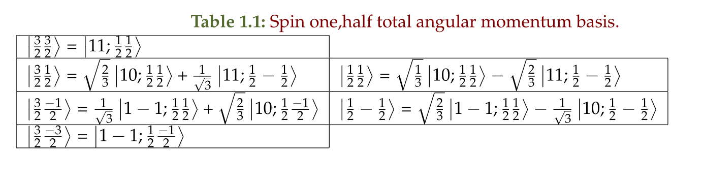
All the basis elements have been determined, and are summarized in table 1.
Example. Spin two, spin one.
With \( j_1 = 2 \) and \( j_2 = 1 \), we have \( j \in 1,2,3 \), and can proceed the same way as sketched in fig. 2.
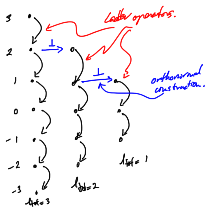
fig. 2. Spin two,one Clebsch-Gordan procedure
References
[1] Jun John Sakurai and Jim J Napolitano. Modern quantum mechanics. Pearson Higher Ed, 2014.