[Click here for a PDF of this post with nicer formatting]
Disclaimer
Peeter’s lecture notes from class. These may be incoherent and rough.
These are notes for the UofT course PHY1520, Graduate Quantum Mechanics, taught by Prof. Paramekanti, covering [1] ch. 5 content.
Perturbation theory
Given a \( 2 \times 2 \) Hamiltonian \( H = H_0 + V \), where
\begin{equation}\label{eqn:qmLecture20:20}
H =
\begin{bmatrix}
a & c \\
c^\conj & b
\end{bmatrix}
\end{equation}
which has eigenvalues
\begin{equation}\label{eqn:qmLecture20:40}
\lambda_\pm = \frac{a + b}{2} \pm \sqrt{ \lr{ \frac{a – b}{2}}^2 + \Abs{c}^2 }.
\end{equation}
If \( c = 0 \),
\begin{equation}\label{eqn:qmLecture20:60}
H_0 =
\begin{bmatrix}
a & 0 \\
0 & b
\end{bmatrix},
\end{equation}
so
\begin{equation}\label{eqn:qmLecture20:80}
V =
\begin{bmatrix}
0 & c \\
c^\conj & 0
\end{bmatrix}.
\end{equation}
Suppose that \( \Abs{c} \ll \Abs{a – b} \), then
\begin{equation}\label{eqn:qmLecture20:100}
\lambda_\pm \approx \frac{a + b}{2} \pm \Abs{ \frac{a – b}{2} } \lr{ 1 + 2 \frac{\Abs{c}^2}{\Abs{a – b}^2} }.
\end{equation}
If \( a > b \), then
\begin{equation}\label{eqn:qmLecture20:120}
\lambda_\pm \approx \frac{a + b}{2} \pm \frac{a – b}{2} \lr{ 1 + 2 \frac{\Abs{c}^2}{\lr{a – b}^2} }.
\end{equation}
\begin{equation}\label{eqn:qmLecture20:140}
\begin{aligned}
\lambda_{+}
&= \frac{a + b}{2} + \frac{a – b}{2} \lr{ 1 + 2 \frac{\Abs{c}^2}{\lr{a – b}^2} } \\
&= a + \lr{a – b} \frac{\Abs{c}^2}{\lr{a – b}^2} \\
&= a + \frac{\Abs{c}^2}{a – b},
\end{aligned}
\end{equation}
and
\begin{equation}\label{eqn:qmLecture20:680}
\begin{aligned}
\lambda_{-}
&= \frac{a + b}{2} – \frac{a – b}{2} \lr{ 1 + 2 \frac{\Abs{c}^2}{\lr{a – b}^2} } \\
&=
b + \lr{a – b} \frac{\Abs{c}^2}{\lr{a – b}^2} \\
&= b + \frac{\Abs{c}^2}{a – b}.
\end{aligned}
\end{equation}
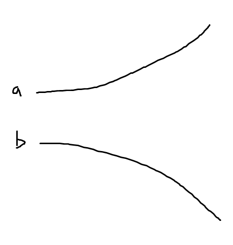
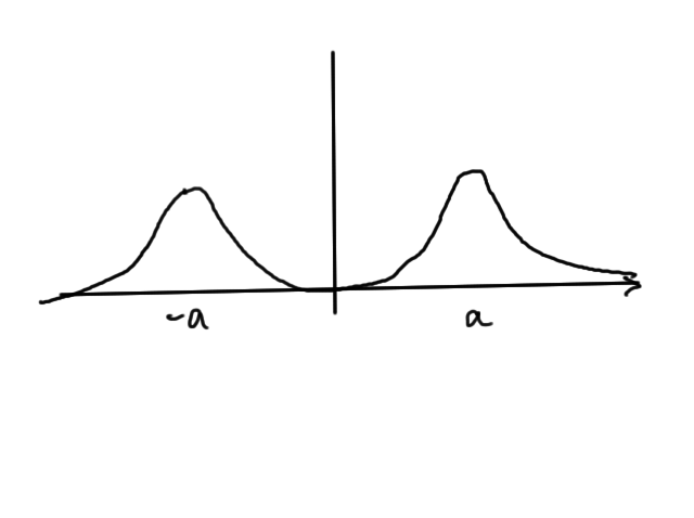
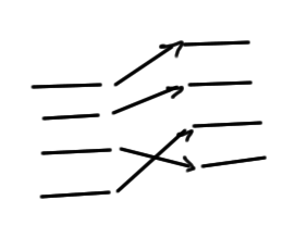
This adiabatic evolution displays a “level repulsion”, quadradic in \( \Abs{c} \) as sketched in fig. 1, and is described as a non-degenerate perbutation.

fig. 1. Adiabatic (non-degenerate) perturbation
If \( \Abs{c} \gg \Abs{a -b} \), then
\begin{equation}\label{eqn:qmLecture20:160}
\begin{aligned}
\lambda_\pm
&= \frac{a + b}{2} \pm \Abs{c} \sqrt{ 1 + \inv{\Abs{c}^2} \lr{ \frac{a – b}{2}}^2 } \\
&\approx \frac{a + b}{2} \pm \Abs{c} \lr{ 1 + \inv{2 \Abs{c}^2} \lr{ \frac{a – b}{2}}^2 } \\
&= \frac{a + b}{2} \pm \Abs{c} \pm \frac{\lr{a – b}^2}{8 \Abs{c}}.
\end{aligned}
\end{equation}
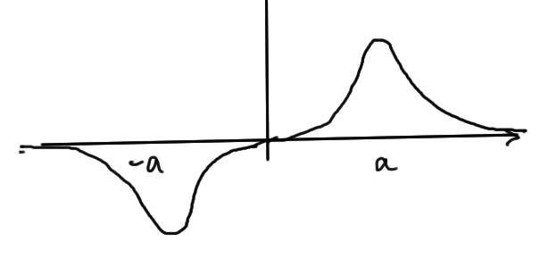
Here we loose the adiabaticity, and have “level repulsion” that is linear in \( \Abs{c} \), as sketched in fig. 2. We no longer have the sign of \( a – b \) in the expansion. This is described as a degenerate perbutation.
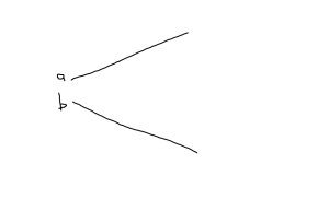
fig. 2. Degenerate perbutation
General non-degenerate perturbation
Given an unperturbed system with solutions of the form
\begin{equation}\label{eqn:qmLecture20:180}
H_0 \ket{n^{(0)}} = E_n^{(0)} \ket{n^{(0)}},
\end{equation}
we want to solve the perturbed Hamiltonian equation
\begin{equation}\label{eqn:qmLecture20:200}
\lr{ H_0 + \lambda V } \ket{ n } = \lr{ E_n^{(0)} + \Delta n } \ket{n}.
\end{equation}
Here \( \Delta n \) is an energy shift as that goes to zero as \( \lambda \rightarrow 0 \). We can write this as
\begin{equation}\label{eqn:qmLecture20:220}
\lr{ E_n^{(0)} – H_0 } \ket{ n } = \lr{ \lambda V – \Delta_n } \ket{n}.
\end{equation}
We are hoping to iterate with application of the inverse to an initial estimate of \( \ket{n} \)
\begin{equation}\label{eqn:qmLecture20:240}
\ket{n} = \lr{ E_n^{(0)} – H_0 }^{-1} \lr{ \lambda V – \Delta_n } \ket{n}.
\end{equation}
This gets us into trouble if \( \lambda \rightarrow 0 \), which can be fixed by using
\begin{equation}\label{eqn:qmLecture20:260}
\ket{n} = \lr{ E_n^{(0)} – H_0 }^{-1} \lr{ \lambda V – \Delta_n } \ket{n} + \ket{ n^{(0)} },
\end{equation}
which can be seen to be a solution to \ref{eqn:qmLecture20:220}. We want to ask if
\begin{equation}\label{eqn:qmLecture20:280}
\lr{ \lambda V – \Delta_n } \ket{n} ,
\end{equation}
contains a bit of \( \ket{ n^{(0)} } \)? To determine this act with \( \bra{n^{(0)}} \) on the left
\begin{equation}\label{eqn:qmLecture20:300}
\begin{aligned}
\bra{ n^{(0)} } \lr{ \lambda V – \Delta_n } \ket{n}
&=
\bra{ n^{(0)} } \lr{ E_n^{(0)} – H_0 } \ket{n} \\
&=
\lr{ E_n^{(0)} – E_n^{(0)} } \braket{n^{(0)}}{n} \\
&=
0.
\end{aligned}
\end{equation}
This shows that \( \ket{n} \) is entirely orthogonal to \( \ket{n^{(0)}} \).
Define a projection operator
\begin{equation}\label{eqn:qmLecture20:320}
P_n = \ket{n^{(0)}}\bra{n^{(0)}},
\end{equation}
which has the idempotent property \( P_n^2 = P_n \) that we expect of a projection operator.
Define a rejection operator
\begin{equation}\label{eqn:qmLecture20:340}
\overline{{P}}_n
= 1 –
\ket{n^{(0)}}\bra{n^{(0)}}
= \sum_{m \ne n}
\ket{m^{(0)}}\bra{m^{(0)}}.
\end{equation}
Because \( \ket{n} \) has no component in the direction \( \ket{n^{(0)}} \), the rejection operator can be inserted much like we normally do with the identity operator, yielding
\begin{equation}\label{eqn:qmLecture20:360}
\ket{n}’ = \lr{ E_n^{(0)} – H_0 }^{-1} \overline{{P}}_n \lr{ \lambda V – \Delta_n } \ket{n} + \ket{ n^{(0)} },
\end{equation}
valid for any initial \( \ket{n} \).
Power series perturbation expansion
Instead of iterating, suppose that the unknown state and unknown energy difference operator can be expanded in a \( \lambda \) power series, say
\begin{equation}\label{eqn:qmLecture20:380}
\ket{n}
=
\ket{n_0}
+ \lambda \ket{n_1}
+ \lambda^2 \ket{n_2}
+ \lambda^3 \ket{n_3} + \cdots
\end{equation}
and
\begin{equation}\label{eqn:qmLecture20:400}
\Delta_{n} = \Delta_{n_0}
+ \lambda \Delta_{n_1}
+ \lambda^2 \Delta_{n_2}
+ \lambda^3 \Delta_{n_3} + \cdots
\end{equation}
We usually interpret functions of operators in terms of power series expansions. In the case of \( \lr{ E_n^{(0)} – H_0 }^{-1} \), we have a concrete interpretation when acting on one of the unpertubed eigenstates
\begin{equation}\label{eqn:qmLecture20:420}
\inv{ E_n^{(0)} – H_0 } \ket{m^{(0)}} =
\inv{ E_n^{(0)} – E_m^0 } \ket{m^{(0)}}.
\end{equation}
This gives
\begin{equation}\label{eqn:qmLecture20:440}
\ket{n}
=
\inv{ E_n^{(0)} – H_0 }
\sum_{m \ne n}
\ket{m^{(0)}}\bra{m^{(0)}}
\lr{ \lambda V – \Delta_n } \ket{n} + \ket{ n^{(0)} },
\end{equation}
or
\begin{equation}\label{eqn:qmLecture20:460}
\boxed{
\ket{n}
=
\ket{ n^{(0)} }
+
\sum_{m \ne n}
\frac{\ket{m^{(0)}}\bra{m^{(0)}}}
{
E_n^{(0)} – E_m^{(0)}
}
\lr{ \lambda V – \Delta_n } \ket{n}.
}
\end{equation}
From \ref{eqn:qmLecture20:220}, note that
\begin{equation}\label{eqn:qmLecture20:500}
\Delta_n =
\frac{\bra{n^{(0)}} \lambda V \ket{n}}{\braket{n^0}{n}},
\end{equation}
however, we will normalize by setting \( \braket{n^0}{n} = 1 \), so
\begin{equation}\label{eqn:qmLecture20:521}
\boxed{
\Delta_n =
\bra{n^{(0)}} \lambda V \ket{n}.
}
\end{equation}
to \( O(\lambda^0) \)
If all \( \lambda^n, n > 0 \) are zero, then we have
\label{eqn:qmLecture20:780}
\begin{equation}\label{eqn:qmLecture20:740}
\ket{n_0}
=
\ket{ n^{(0)} }
+
\sum_{m \ne n}
\frac{\ket{m^{(0)}}\bra{m^{(0)}}}
{
E_n^{(0)} – E_m^{(0)}
}
\lr{ – \Delta_{n_0} } \ket{n_0}
\end{equation}
\begin{equation}\label{eqn:qmLecture20:800}
\Delta_{n_0} \braket{n^{(0)}}{n_0} = 0
\end{equation}
so
\begin{equation}\label{eqn:qmLecture20:540}
\begin{aligned}
\ket{n_0} &= \ket{n^{(0)}} \\
\Delta_{n_0} &= 0.
\end{aligned}
\end{equation}
to \( O(\lambda^1) \)
Requiring identity for all \( \lambda^1 \) terms means
\begin{equation}\label{eqn:qmLecture20:760}
\ket{n_1} \lambda
=
\sum_{m \ne n}
\frac{\ket{m^{(0)}}\bra{m^{(0)}}}
{
E_n^{(0)} – E_m^{(0)}
}
\lr{ \lambda V – \Delta_{n_1} \lambda } \ket{n_0},
\end{equation}
so
\begin{equation}\label{eqn:qmLecture20:560}
\ket{n_1}
=
\sum_{m \ne n}
\frac{
\ket{m^{(0)}} \bra{ m^{(0)}}
}
{
E_n^{(0)} – E_m^{(0)}
}
\lr{ V – \Delta_{n_1} } \ket{n_0}.
\end{equation}
With the assumption that \( \ket{n^{(0)}} \) is normalized, and with the shorthand
\begin{equation}\label{eqn:qmLecture20:600}
V_{m n} = \bra{ m^{(0)}} V \ket{n^{(0)}},
\end{equation}
that is
\begin{equation}\label{eqn:qmLecture20:580}
\begin{aligned}
\ket{n_1}
&=
\sum_{m \ne n}
\frac{
\ket{m^{(0)}}
}
{
E_n^{(0)} – E_m^{(0)}
}
V_{m n}
\\
\Delta_{n_1} &= \bra{ n^{(0)} } V \ket{ n^0} = V_{nn}.
\end{aligned}
\end{equation}
to \( O(\lambda^2) \)
The second order perturbation states are found by selecting only the \( \lambda^2 \) contributions to
\begin{equation}\label{eqn:qmLecture20:820}
\lambda^2 \ket{n_2}
=
\sum_{m \ne n}
\frac{\ket{m^{(0)}}\bra{m^{(0)}}}
{
E_n^{(0)} – E_m^{(0)}
}
\lr{ \lambda V – (\lambda \Delta_{n_1} + \lambda^2 \Delta_{n_2}) }
\lr{
\ket{n_0}
+ \lambda \ket{n_1}
}.
\end{equation}
Because \( \ket{n_0} = \ket{n^{(0)}} \), the \( \lambda^2 \Delta_{n_2} \) is killed, leaving
\begin{equation}\label{eqn:qmLecture20:840}
\begin{aligned}
\ket{n_2}
&=
\sum_{m \ne n}
\frac{\ket{m^{(0)}}\bra{m^{(0)}}}
{
E_n^{(0)} – E_m^{(0)}
}
\lr{ V – \Delta_{n_1} }
\ket{n_1} \\
&=
\sum_{m \ne n}
\frac{\ket{m^{(0)}}\bra{m^{(0)}}}
{
E_n^{(0)} – E_m^{(0)}
}
\lr{ V – \Delta_{n_1} }
\sum_{l \ne n}
\frac{
\ket{l^{(0)}}
}
{
E_n^{(0)} – E_l^{(0)}
}
V_{l n},
\end{aligned}
\end{equation}
which can be written as
\begin{equation}\label{eqn:qmLecture20:620}
\ket{n_2}
=
\sum_{l,m \ne n}
\ket{m^{(0)}}
\frac{V_{m l} V_{l n}}
{
\lr{ E_n^{(0)} – E_m^{(0)} }
\lr{ E_n^{(0)} – E_l^{(0)} }
}
–
\sum_{m \ne n}
\ket{m^{(0)}}
\frac{V_{n n} V_{m n}}
{
\lr{ E_n^{(0)} – E_m^{(0)} }^2
}.
\end{equation}
For the second energy perturbation we have
\begin{equation}\label{eqn:qmLecture20:860}
\lambda^2 \Delta_{n_2} =
\bra{n^{(0)}} \lambda V \lr{ \lambda \ket{n_1} },
\end{equation}
or
\begin{equation}\label{eqn:qmLecture20:880}
\begin{aligned}
\Delta_{n_2}
&=
\bra{n^{(0)}} V \ket{n_1} \\
&=
\bra{n^{(0)}} V
\sum_{m \ne n}
\frac{
\ket{m^{(0)}}
}
{
E_n^{(0)} – E_m^{(0)}
}
V_{m n}.
\end{aligned}
\end{equation}
That is
\begin{equation}\label{eqn:qmLecture20:900}
\Delta_{n_2}
=
\sum_{m \ne n} \frac{V_{n m} V_{m n} }{E_n^{(0)} – E_m^{(0)}}.
\end{equation}
to \( O(\lambda^3) \)
Similarily, it can be shown that
\begin{equation}\label{eqn:qmLecture20:640}
\Delta_{n_3} =
\sum_{l, m \ne n} \frac{V_{n m} V_{m l} V_{l n} }{
\lr{ E_n^{(0)} – E_m^{(0)} }
\lr{ E_n^{(0)} – E_l^{(0)} }
}
–
\sum_{ m \ne n} \frac{V_{n m} V_{n n} V_{m n} }{
\lr{ E_n^{(0)} – E_m^{(0)} }^2
}.
\end{equation}
In general, the energy perturbation is given by
\begin{equation}\label{eqn:qmLecture20:660}
\Delta_n^{(l)} = \bra{n^{(0)}} V \ket{n^{(l-1)}}.
\end{equation}
References
[1] Jun John Sakurai and Jim J Napolitano. Modern quantum mechanics. Pearson Higher Ed, 2014.
Like this:
Like Loading...