bra

PHY2403 (QFT I). Pondering the ground state bra formula.

November 5, 2018 phy2403 , ,

[Click here for a PDF of this post with nicer formatting]

In lecture 14 we found

\begin{equation}\label{eqn:qftLecture15:60}
\ket{\Omega}
=
\evalbar{
\frac{ U(t_0, -T) \ket{0} }
{
e^{-i E_0(T – t_0)} \braket{\Omega}{0}
}
}{T \rightarrow \infty(1 – i \epsilon)},
\end{equation}
and it was stated that we can also show that
\begin{equation}\label{eqn:qftLecture15:80}
\bra{\Omega}
=
\evalbar{
\frac{ \bra{0} U(T, t_0) }
{
e^{-i E_0(T – t_0)} \braket{0}{\Omega}
}
}{T \rightarrow \infty(1 – i \epsilon)}.
\end{equation}

This second statement is actually not obvious since
\begin{equation}\label{eqn:braOmega:100}
\lr{
\frac{ U(t_0, -T) \ket{0} }
{
e^{-i E_0(T – t_0)} \braket{\Omega}{0}
}
}^\dagger
=
\frac{ \bra{0} U(-T, t_0) \ket{0} }
{
e^{+i E_0(T – t_0)} \braket{0}{\Omega}
}
\end{equation}

My first thought was that I’d written down \ref{eqn:qftLecture15:80} in my notes wrong, but this is actually also consistent with [1], which our Prof is following loosely (i.e. he is explicitly filling in many of the holes in that dense little 800 page book).

The resolution of this inconsistency is that the limit point \( \infty(1 – i \epsilon) \) doesn’t work if you just conjugate, and you’d also have to conjugate that limit, so while
\ref{eqn:braOmega:100} is correct, it is only part of the story, and should really be stated as
\begin{equation}\label{eqn:braOmega:120}
\bra{\Omega}
=
\evalbar{
\frac{ \bra{0} U(-T, t_0) \ket{0} }
{
e^{+i E_0(T – t_0)} \braket{0}{\Omega}
}
}{T \rightarrow \infty(1 + i \epsilon)}.
\end{equation}
This is awkward because now our expressions for \( \bra{\Omega} \) and \( \ket{\Omega} \) approach \( T \) from different directions, and we want to evaluate both with a single limiting argument.

To resolve this, we really have to start back with the identity expansion we used in lecture 14
\begin{equation}\label{eqn:braOmega:140}
\begin{aligned}
\bra{0} e^{-i H T}
&=
\lr{
\braket{0}{\Omega}\bra{\Omega}
+ {\int\kern-1em\sum}_n \braket{0}{n} \bra{n}
}
e^{-i H T} \\
&=
\braket{0}{\Omega}\bra{\Omega}
e^{-i E_0 T}
+ {\int\kern-1em\sum}_n \braket{0}{n} \bra{n} e^{-i E_n T}.
\end{aligned}
\end{equation}
We argued (as does the text) that approaching to as \( T( 1 – i \epsilon) \) kills off the energetic states since
\begin{equation}\label{eqn:braOmega:160}
\bra{n} e^{-i E_n T}
\rightarrow
\bra{n} e^{-i E_n T} e^{-E_n T \epsilon}
\end{equation}
and the exponential damping factor is smaller for each \( E_n > E_0 \), so it can be neglected in the large \( T \) limit, leaving
\begin{equation}\label{eqn:braOmega:180}
\bra{0} e^{-i H T}
=
\lim_{T \rightarrow \infty(1 – i \epsilon)}
\braket{0}{\Omega}\bra{\Omega}.
\end{equation}
As we did for \( \ket{\Omega} \) we can shift the large time \( T \) by a small constant (this time \( -t_0 \) instead of \( t_0 \)), to give
\begin{equation}\label{eqn:braOmega:200}
\begin{aligned}
\bra{\Omega}
&=
\lim_{T \rightarrow \infty(1 – i \epsilon)}
\frac{ \bra{0} e^{-i H T} }
{
\braket{0}{\Omega} e^{-i E_0 T}
} \\
&\approx
\lim_{T \rightarrow \infty(1 – i \epsilon)}
\frac{ \bra{0} e^{-i H (T – t_0)} }
{
\braket{0}{\Omega} e^{-i E_0 (T – t_0)}
} \\
&=
\lim_{T \rightarrow \infty(1 – i \epsilon)}
\frac{ \bra{0} e^{i H_0( T – t_0)} e^{-i H (T – t_0)} }
{
\braket{0}{\Omega} e^{-i E_0 (T – t_0)}
} \\
&=
\lim_{T \rightarrow \infty(1 – i \epsilon)}
\frac{ \bra{0} U(T, t_0) }
{
\braket{0}{\Omega} e^{-i E_0 (T – t_0)}
},
\end{aligned}
\end{equation}
where the projective property \( \bra{0} e^{i H_0 \alpha} = \bra{0} \) has been used to insert a no-op (i.e. \( \bra{0} H_0 = 0 \)). This recovers the result stated in class (also: eq. (4.29) in the text.)

References

[1] Michael E Peskin and Daniel V Schroeder. An introduction to Quantum Field Theory. Westview, 1995.
Plane wave ground state expectation for SHO

October 18, 2015 phy1520 , , , , , , , , , , ,

[Click here for a PDF of this post with nicer formatting]

Problem [1] 2.18 is, for a 1D SHO, show that

\begin{equation}\label{eqn:exponentialExpectationGroundState:20}
\bra{0} e^{i k x} \ket{0} = \exp\lr{ -k^2 \bra{0} x^2 \ket{0}/2 }.
\end{equation}

Despite the simple appearance of this problem, I found this quite involved to show. To do so, start with a series expansion of the expectation

\begin{equation}\label{eqn:exponentialExpectationGroundState:40}
\bra{0} e^{i k x} \ket{0}
=
\sum_{m=0}^\infty \frac{(i k)^m}{m!} \bra{0} x^m \ket{0}.
\end{equation}

Let

\begin{equation}\label{eqn:exponentialExpectationGroundState:60}
X = \lr{ a + a^\dagger },
\end{equation}

so that

\begin{equation}\label{eqn:exponentialExpectationGroundState:80}
x
= \sqrt{\frac{\Hbar}{2 \omega m}} X
= \frac{x_0}{\sqrt{2}} X.
\end{equation}

Consider the first few values of \( \bra{0} X^n \ket{0} \)

\begin{equation}\label{eqn:exponentialExpectationGroundState:100}
\begin{aligned}
\bra{0} X \ket{0}
&=
\bra{0} \lr{ a + a^\dagger } \ket{0} \\
&=
\braket{0}{1} \\
&=
0,
\end{aligned}
\end{equation}

\begin{equation}\label{eqn:exponentialExpectationGroundState:120}
\begin{aligned}
\bra{0} X^2 \ket{0}
&=
\bra{0} \lr{ a + a^\dagger }^2 \ket{0} \\
&=
\braket{1}{1} \\
&=
1,
\end{aligned}
\end{equation}

\begin{equation}\label{eqn:exponentialExpectationGroundState:140}
\begin{aligned}
\bra{0} X^3 \ket{0}
&=
\bra{0} \lr{ a + a^\dagger }^3 \ket{0} \\
&=
\bra{1} \lr{ \sqrt{2} \ket{2} + \ket{0} } \\
&=
0.
\end{aligned}
\end{equation}

Whenever the power \( n \) in \( X^n \) is even, the braket can be split into a bra that has only contributions from odd eigenstates and a ket with even eigenstates. We conclude that \( \bra{0} X^n \ket{0} = 0 \) when \( n \) is odd.

Noting that \( \bra{0} x^2 \ket{0} = \ifrac{x_0^2}{2} \), this leaves

\begin{equation}\label{eqn:exponentialExpectationGroundState:160}
\begin{aligned}
\bra{0} e^{i k x} \ket{0}
&=
\sum_{m=0}^\infty \frac{(i k)^{2 m}}{(2 m)!} \bra{0} x^{2m} \ket{0} \\
&=
\sum_{m=0}^\infty \frac{(i k)^{2 m}}{(2 m)!} \lr{ \frac{x_0^2}{2} }^m \bra{0} X^{2m} \ket{0} \\
&=
\sum_{m=0}^\infty \frac{1}{(2 m)!} \lr{ -k^2 \bra{0} x^2 \ket{0} }^m \bra{0} X^{2m} \ket{0}.
\end{aligned}
\end{equation}

This problem is now reduced to showing that

\begin{equation}\label{eqn:exponentialExpectationGroundState:180}
\frac{1}{(2 m)!} \bra{0} X^{2m} \ket{0} = \inv{m! 2^m},
\end{equation}

or

\begin{equation}\label{eqn:exponentialExpectationGroundState:200}
\begin{aligned}
\bra{0} X^{2m} \ket{0}
&= \frac{(2m)!}{m! 2^m} \\
&= \frac{ (2m)(2m-1)(2m-2) \cdots (2)(1) }{2^m m!} \\
&= \frac{ 2^m (m)(2m-1)(m-1)(2m-3)(m-2) \cdots (2)(3)(1)(1) }{2^m m!} \\
&= (2m-1)!!,
\end{aligned}
\end{equation}

where \( n!! = n(n-2)(n-4)\cdots \).

It looks like \( \bra{0} X^{2m} \ket{0} \) can be expanded by inserting an identity operator and proceeding recursively, like

\begin{equation}\label{eqn:exponentialExpectationGroundState:220}
\begin{aligned}
\bra{0} X^{2m} \ket{0}
&=
\bra{0} X^2 \lr{ \sum_{n=0}^\infty \ket{n}\bra{n} } X^{2m-2} \ket{0} \\
&=
\bra{0} X^2 \lr{ \ket{0}\bra{0} + \ket{2}\bra{2} } X^{2m-2} \ket{0} \\
&=
\bra{0} X^{2m-2} \ket{0} + \bra{0} X^2 \ket{2} \bra{2} X^{2m-2} \ket{0}.
\end{aligned}
\end{equation}

This has made use of the observation that \( \bra{0} X^2 \ket{n} = 0 \) for all \( n \ne 0,2 \). The remaining term includes the factor

\begin{equation}\label{eqn:exponentialExpectationGroundState:240}
\begin{aligned}
\bra{0} X^2 \ket{2}
&=
\bra{0} \lr{a + a^\dagger}^2 \ket{2} \\
&=
\lr{ \bra{0} + \sqrt{2} \bra{2} } \ket{2} \\
&=
\sqrt{2},
\end{aligned}
\end{equation}

Since \( \sqrt{2} \ket{2} = \lr{a^\dagger}^2 \ket{0} \), the expectation of interest can be written

\begin{equation}\label{eqn:exponentialExpectationGroundState:260}
\bra{0} X^{2m} \ket{0}
=
\bra{0} X^{2m-2} \ket{0} + \bra{0} a^2 X^{2m-2} \ket{0}.
\end{equation}

How do we expand the second term. Let’s look at how \( a \) and \( X \) commute

\begin{equation}\label{eqn:exponentialExpectationGroundState:280}
\begin{aligned}
a X
&=
\antisymmetric{a}{X} + X a \\
&=
\antisymmetric{a}{a + a^\dagger} + X a \\
&=
\antisymmetric{a}{a^\dagger} + X a \\
&=
1 + X a,
\end{aligned}
\end{equation}

\begin{equation}\label{eqn:exponentialExpectationGroundState:300}
\begin{aligned}
a^2 X
&=
a \lr{ a X } \\
&=
a \lr{ 1 + X a } \\
&=
a + a X a \\
&=
a + \lr{ 1 + X a } a \\
&=
2 a + X a^2.
\end{aligned}
\end{equation}

Proceeding to expand \( a^2 X^n \) we find
\begin{equation}\label{eqn:exponentialExpectationGroundState:320}
\begin{aligned}
a^2 X^3 &= 6 X + 6 X^2 a + X^3 a^2 \\
a^2 X^4 &= 12 X^2 + 8 X^3 a + X^4 a^2 \\
a^2 X^5 &= 20 X^3 + 10 X^4 a + X^5 a^2 \\
a^2 X^6 &= 30 X^4 + 12 X^5 a + X^6 a^2.
\end{aligned}
\end{equation}

It appears that we have
\begin{equation}\label{eqn:exponentialExpectationGroundState:340}
\antisymmetric{a^2 X^n}{X^n a^2} = \beta_n X^{n-2} + 2 n X^{n-1} a,
\end{equation}

where

\begin{equation}\label{eqn:exponentialExpectationGroundState:360}
\beta_n = \beta_{n-1} + 2 (n-1),
\end{equation}

and \( \beta_2 = 2 \). Some goofing around shows that \( \beta_n = n(n-1) \), so the induction hypothesis is

\begin{equation}\label{eqn:exponentialExpectationGroundState:380}
\antisymmetric{a^2 X^n}{X^n a^2} = n(n-1) X^{n-2} + 2 n X^{n-1} a.
\end{equation}

Let’s check the induction
\begin{equation}\label{eqn:exponentialExpectationGroundState:400}
\begin{aligned}
a^2 X^{n+1}
&=
a^2 X^{n} X \\
&=
\lr{ n(n-1) X^{n-2} + 2 n X^{n-1} a + X^n a^2 } X \\
&=
n(n-1) X^{n-1} + 2 n X^{n-1} a X + X^n a^2 X \\
&=
n(n-1) X^{n-1} + 2 n X^{n-1} \lr{ 1 + X a } + X^n \lr{ 2 a + X a^2 } \\
&=
n(n-1) X^{n-1} + 2 n X^{n-1} + 2 n X^{n} a
+ 2 X^n a
+ X^{n+1} a^2 \\
&=
X^{n+1} a^2 + (2 + 2 n) X^{n} a + \lr{ 2 n + n(n-1) } X^{n-1} \\
&=
X^{n+1} a^2 + 2(n + 1) X^{n} a + (n+1) n X^{n-1},
\end{aligned}
\end{equation}

which concludes the induction, giving

\begin{equation}\label{eqn:exponentialExpectationGroundState:420}
\bra{ 0 } a^2 X^{n} \ket{0 } = n(n-1) \bra{0} X^{n-2} \ket{0},
\end{equation}

and

\begin{equation}\label{eqn:exponentialExpectationGroundState:440}
\bra{0} X^{2m} \ket{0}
=
\bra{0} X^{2m-2} \ket{0} + (2m-2)(2m-3) \bra{0} X^{2m-4} \ket{0}.
\end{equation}

Let

\begin{equation}\label{eqn:exponentialExpectationGroundState:460}
\sigma_{n} = \bra{0} X^n \ket{0},
\end{equation}

so that the recurrence relation, for \( 2n \ge 4 \) is

\begin{equation}\label{eqn:exponentialExpectationGroundState:480}
\sigma_{2n} = \sigma_{2n -2} + (2n-2)(2n-3) \sigma_{2n -4}
\end{equation}

We want to show that this simplifies to

\begin{equation}\label{eqn:exponentialExpectationGroundState:500}
\sigma_{2n} = (2n-1)!!
\end{equation}

The first values are

\begin{equation}\label{eqn:exponentialExpectationGroundState:540}
\sigma_0 = \bra{0} X^0 \ket{0} = 1
\end{equation}
\begin{equation}\label{eqn:exponentialExpectationGroundState:560}
\sigma_2 = \bra{0} X^2 \ket{0} = 1
\end{equation}

which gives us the right result for the first term in the induction

\begin{equation}\label{eqn:exponentialExpectationGroundState:580}
\begin{aligned}
\sigma_4
&= \sigma_2 + 2 \times 1 \times \sigma_0 \\
&= 1 + 2 \\
&= 3!!
\end{aligned}
\end{equation}

For the general induction term, consider

\begin{equation}\label{eqn:exponentialExpectationGroundState:600}
\begin{aligned}
\sigma_{2n + 2}
&= \sigma_{2n} + 2 n (2n – 1) \sigma_{2n -2} \\
&= (2n-1)!! + 2n ( 2n – 1) (2n -3)!! \\
&= (2n + 1) (2n -1)!! \\
&= (2n + 1)!!,
\end{aligned}
\end{equation}

which completes the final induction. That was also the last thing required to complete the proof, so we are done!

References

[1] Jun John Sakurai and Jim J Napolitano. Modern quantum mechanics. Pearson Higher Ed, 2014.

PHY1520H Graduate Quantum Mechanics. Lecture 3: Density matrix (cont.). Taught by Prof. Arun Paramekanti

September 24, 2015 phy1520 , , , , , , , , ,

[Click here for a PDF of this post with nicer formatting]

Disclaimer

Peeter’s lecture notes from class. These may be incoherent and rough.

These are notes for the UofT course PHY1520, Graduate Quantum Mechanics, taught by Prof. Paramekanti, covering [1] chap. 3 content.

Density matrix (cont.)

An example of a partitioned system with four total states (two spin 1/2 particles) is sketched in fig. 1.

fig. 1.  Two spins

fig. 1. Two spins

An example of a partitioned system with eight total states (three spin 1/2 particles) is sketched in fig. 2.

fig. 2.  Three spins

fig. 2. Three spins

The density matrix

\begin{equation}\label{eqn:qmLecture3:20}
\hat{\rho} = \ket{\Psi}\bra{\Psi}
\end{equation}

is clearly an operator as can be seen by applying it to a state

\begin{equation}\label{eqn:qmLecture3:40}
\hat{\rho} \ket{\phi} = \ket{\Psi} \lr{ \braket{ \Psi }{\phi} }.
\end{equation}

The quantity in braces is just a complex number.

After expanding the pure state \( \ket{\Psi} \) in terms of basis states for each of the two partitions

\begin{equation}\label{eqn:qmLecture3:60}
\ket{\Psi}
= \sum_{m,n} C_{m, n} \ket{m}_{\textrm{L}} \ket{n}_{\textrm{R}},
\end{equation}

With \( \textrm{L} \) and \( \textrm{R} \) implied for \( \ket{m}, \ket{n} \) indexed states respectively, this can be written

\begin{equation}\label{eqn:qmLecture3:460}
\ket{\Psi}
= \sum_{m,n} C_{m, n} \ket{m} \ket{n}.
\end{equation}

The density operator is

\begin{equation}\label{eqn:qmLecture3:80}
\hat{\rho} =
\sum_{m,n}
C_{m, n}
C_{m’, n’}^\conj
\ket{m} \ket{n}
\sum_{m’,n’}
\bra{m’} \bra{n’}.
\end{equation}

Suppose we trace over the right partition of the state space, defining such a trace as the reduced density operator \( \hat{\rho}_{\textrm{red}} \)

\begin{equation}\label{eqn:qmLecture3:100}
\begin{aligned}
\hat{\rho}_{\textrm{red}}
&\equiv
\textrm{Tr}_{\textrm{R}}(\hat{\rho}) \\
&= \sum_{\tilde{n}} \bra{\tilde{n}} \hat{\rho} \ket{ \tilde{n}} \\
&= \sum_{\tilde{n}}
\bra{\tilde{n} }
\lr{
\sum_{m,n}
C_{m, n}
\ket{m} \ket{n}
}
\lr{
\sum_{m’,n’}
C_{m’, n’}^\conj
\bra{m’} \bra{n’}
}
\ket{ \tilde{n} } \\
&=
\sum_{\tilde{n}}
\sum_{m,n}
\sum_{m’,n’}
C_{m, n}
C_{m’, n’}^\conj
\ket{m} \delta_{\tilde{n} n}
\bra{m’ }
\delta_{ \tilde{n} n’ } \\
&=
\sum_{\tilde{n}, m, m’}
C_{m, \tilde{n}}
C_{m’, \tilde{n}}^\conj
\ket{m} \bra{m’ }
\end{aligned}
\end{equation}

Computing the matrix element of \( \hat{\rho}_{\textrm{red}} \), we have

\begin{equation}\label{eqn:qmLecture3:120}
\begin{aligned}
\bra{\tilde{m}} \hat{\rho}_{\textrm{red}} \ket{\tilde{m}}
&=
\sum_{m, m’, \tilde{n}} C_{m, \tilde{n}} C_{m’, \tilde{n}}^\conj \braket{ \tilde{m}}{m} \braket{m’}{\tilde{m}} \\
&=
\sum_{\tilde{n}} \Abs{C_{\tilde{m}, \tilde{n}} }^2.
\end{aligned}
\end{equation}

This is the probability that the left partition is in state \( \tilde{m} \).

Average of an observable

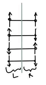
Suppose we have two spin half particles. For such a system the total magnetization is

\begin{equation}\label{eqn:qmLecture3:140}
S_{\textrm{Total}} =
S_1^z
+
S_1^z,
\end{equation}

as sketched in fig. 3.

fig. 3.  Magnetic moments from two spins.

fig. 3. Magnetic moments from two spins.

The average of some observable is

\begin{equation}\label{eqn:qmLecture3:160}
\expectation{\hatA}
= \sum_{m, n, m’, n’} C_{m, n}^\conj C_{m’, n’}
\bra{m}\bra{n} \hatA \ket{n’} \ket{m’}.
\end{equation}

Consider the trace of the density operator observable product

\begin{equation}\label{eqn:qmLecture3:180}
\textrm{Tr}( \hat{\rho} \hatA )
= \sum_{m, n} \braket{m n}{\Psi} \bra{\Psi} \hatA \ket{m, n}.
\end{equation}

Let

\begin{equation}\label{eqn:qmLecture3:200}
\ket{\Psi} = \sum_{m, n} C_{m n} \ket{m, n},
\end{equation}

so that

\begin{equation}\label{eqn:qmLecture3:220}
\begin{aligned}
\textrm{Tr}( \hat{\rho} \hatA )
&= \sum_{m, n, m’, n’, m”, n”} C_{m’, n’} C_{m”, n”}^\conj
\braket{m n}{m’, n’} \bra{m”, n”} \hatA \ket{m, n} \\
&= \sum_{m, n, m”, n”} C_{m, n} C_{m”, n”}^\conj
\bra{m”, n”} \hatA \ket{m, n}.
\end{aligned}
\end{equation}

This is just

\begin{equation}\label{eqn:qmLecture3:240}
\boxed{
\bra{\Psi} \hatA \ket{\Psi} = \textrm{Tr}( \hat{\rho} \hatA ).
}
\end{equation}

Left observables

Consider

\begin{equation}\label{eqn:qmLecture3:260}
\begin{aligned}
\bra{\Psi} \hatA_{\textrm{L}} \ket{\Psi}
&= \textrm{Tr}(\hat{\rho} \hatA_{\textrm{L}}) \\
&=
\textrm{Tr}_{\textrm{L}}
\textrm{Tr}_{\textrm{R}}
(\hat{\rho} \hatA_{\textrm{L}}) \\
&=
\textrm{Tr}_{\textrm{L}}
\lr{
\lr{
\textrm{Tr}_{\textrm{R}} \hat{\rho}
}
\hatA_{\textrm{L}})
} \\
&=
\textrm{Tr}_{\textrm{L}}
\lr{
\hat{\rho}_{\textrm{red}}
\hatA_{\textrm{L}})
}.
\end{aligned}
\end{equation}

We see

\begin{equation}\label{eqn:qmLecture3:280}
\bra{\Psi} \hatA_{\textrm{L}} \ket{\Psi}
=
\textrm{Tr}_{\textrm{L}} \lr{ \hat{\rho}_{\textrm{red}, \textrm{L}} \hatA_{\textrm{L}} }.
\end{equation}

We find that we don’t need to know the state of the complete system to answer questions about portions of the system, but instead just need \( \hat{\rho} \), a “probability operator” that provides all the required information about the partitioning of the system.

Pure states vs. mixed states

For pure states we can assign a state vector and talk about reduced scenarios. For mixed states we must work with reduced density matrix.

Example: Two particle spin half pure states

Consider

\begin{equation}\label{eqn:qmLecture3:300}
\ket{\psi_1} = \inv{\sqrt{2}} \lr{ \ket{ \uparrow \downarrow } – \ket{ \downarrow \uparrow } }
\end{equation}

\begin{equation}\label{eqn:qmLecture3:320}
\ket{\psi_2} = \inv{\sqrt{2}} \lr{ \ket{ \uparrow \downarrow } + \ket{ \uparrow \uparrow } }.
\end{equation}

For the first pure state the density operator is
\begin{equation}\label{eqn:qmLecture3:360}
\hat{\rho} = \inv{2}
\lr{ \ket{ \uparrow \downarrow } – \ket{ \downarrow \uparrow } }
\lr{ \bra{ \uparrow \downarrow } – \bra{ \downarrow \uparrow } }
\end{equation}

What are the reduced density matrices?

\begin{equation}\label{eqn:qmLecture3:340}
\begin{aligned}
\hat{\rho}_{\textrm{L}}
&= \textrm{Tr}_{\textrm{R}} \lr{ \hat{\rho} } \\
&=
\inv{2} (-1)(-1) \ket{\downarrow}\bra{\downarrow}
+\inv{2} (+1)(+1) \ket{\uparrow}\bra{\uparrow},
\end{aligned}
\end{equation}

so the matrix representation of this reduced density operator is

\begin{equation}\label{eqn:qmLecture3:380}
\hat{\rho}_{\textrm{L}}
=
\inv{2}
\begin{bmatrix}
1 & 0 \\
0 & 1
\end{bmatrix}.
\end{equation}

For the second pure state the density operator is
\begin{equation}\label{eqn:qmLecture3:400}
\hat{\rho} = \inv{2}
\lr{ \ket{ \uparrow \downarrow } + \ket{ \uparrow \uparrow } }
\lr{ \bra{ \uparrow \downarrow } + \bra{ \uparrow \uparrow } }.
\end{equation}

This has a reduced density matrice

\begin{equation}\label{eqn:qmLecture3:420}
\begin{aligned}
\hat{\rho}_{\textrm{L}}
&= \textrm{Tr}_{\textrm{R}} \lr{ \hat{\rho} } \\
&=
\inv{2} \ket{\uparrow}\bra{\uparrow}
+\inv{2} \ket{\uparrow}\bra{\uparrow} \\
&=
\ket{\uparrow}\bra{\uparrow} .
\end{aligned}
\end{equation}

This has a matrix representation

\begin{equation}\label{eqn:qmLecture3:440}
\hat{\rho}_{\textrm{L}}
=
\begin{bmatrix}
1 & 0 \\
0 & 0
\end{bmatrix}.
\end{equation}

In this second example, we have more information about the left partition. That will be seen as a zero entanglement entropy in the problem set. In contrast we have less information about the first state, and will find a non-zero positive entanglement entropy in that case.

References

[1] Jun John Sakurai and Jim J Napolitano. Modern quantum mechanics. Pearson Higher Ed, 2014.

PHY1520H Graduate Quantum Mechanics. Lecture 1: Lighting review. Taught by Prof. Arun Paramekanti

September 17, 2015 phy1520 , , , , , , , , , , , , , ,

[Click here for a PDF of this post with nicer formatting]

Disclaimer

Peeter’s lecture notes from class. These may be incoherent and rough.

These are notes for the UofT course PHY1520, Graduate Quantum Mechanics, taught by Prof. Paramekanti, covering [1] chap. 1 content.

Classical mechanics

We’ll be talking about one body physics for most of this course. In classical mechanics we can figure out the particle trajectories using both of \( (\Br, \Bp \), where

\begin{equation}\label{eqn:qmLecture1:20}
\begin{aligned}
\ddt{\Br} &= \inv{m} \Bp \\
\ddt{\Bp} &= \spacegrad V
\end{aligned}
\end{equation}

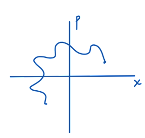
A two dimensional phase space as sketched in fig. 1 shows the trajectory of a point particle subject to some equations of motion

lectureOnePhaseSpaceClassicalFig1

fig. 1. One dimensional classical phase space example

Quantum mechanics

For this lecture, we’ll work with natural units, setting

\begin{equation}\label{eqn:qmLecture1:480}
\boxed{
\Hbar = 1.
}
\end{equation}

In QM we are no longer allowed to think of position and momentum, but have to start asking about state vectors \( \ket{\Psi} \).

We’ll consider the state vector with respect to some basis, for example, in a position basis, we write

\begin{equation}\label{eqn:qmLecture1:40}
\braket{ x }{\Psi } = \Psi(x),
\end{equation}

a complex numbered “wave function”, the probability amplitude for a particle in \( \ket{\Psi} \) to be in the vicinity of \( x \).

We could also consider the state in a momentum basis

\begin{equation}\label{eqn:qmLecture1:60}
\braket{ p }{\Psi } = \Psi(p),
\end{equation}

a probability amplitude with respect to momentum \( p \).

More precisely,

\begin{equation}\label{eqn:qmLecture1:80}
\Abs{\Psi(x)}^2 dx \ge 0
\end{equation}

is the probability of finding the particle in the range \( (x, x + dx ) \). To have meaning as a probability, we require

\begin{equation}\label{eqn:qmLecture1:100}
\int_{-\infty}^\infty \Abs{\Psi(x)}^2 dx = 1.
\end{equation}

The average position can be calculated using this probability density function. For example

\begin{equation}\label{eqn:qmLecture1:120}
\expectation{x} = \int_{-\infty}^\infty \Abs{\Psi(x)}^2 x dx,
\end{equation}

or
\begin{equation}\label{eqn:qmLecture1:140}
\expectation{f(x)} = \int_{-\infty}^\infty \Abs{\Psi(x)}^2 f(x) dx.
\end{equation}

Similarly, calculation of an average of a function of momentum can be expressed as

\begin{equation}\label{eqn:qmLecture1:160}
\expectation{f(p)} = \int_{-\infty}^\infty \Abs{\Psi(p)}^2 f(p) dp.
\end{equation}

Transformation from a position to momentum basis

We have a problem, if we which to compute an average in momentum space such as \( \expectation{p} \), when given a wavefunction \( \Psi(x) \).

How do we convert

\begin{equation}\label{eqn:qmLecture1:180}
\Psi(p)
\stackrel{?}{\leftrightarrow}
\Psi(x),
\end{equation}

or equivalently
\begin{equation}\label{eqn:qmLecture1:200}
\braket{p}{\Psi}
\stackrel{?}{\leftrightarrow}
\braket{x}{\Psi}.
\end{equation}

Such a conversion can be performed by virtue of an the assumption that we have a complete orthonormal basis, for which we can introduce identity operations such as

\begin{equation}\label{eqn:qmLecture1:220}
\int_{-\infty}^\infty dp \ket{p}\bra{p} = 1,
\end{equation}

or
\begin{equation}\label{eqn:qmLecture1:240}
\int_{-\infty}^\infty dx \ket{x}\bra{x} = 1
\end{equation}

Some interpretations:

  1. \( \ket{x_0} \leftrightarrow \text{sits at} x = x_0 \)
  2. \( \braket{x}{x’} \leftrightarrow \delta(x – x’) \)
  3. \( \braket{p}{p’} \leftrightarrow \delta(p – p’) \)
  4. \( \braket{x}{p’} = \frac{e^{i p x}}{\sqrt{V}} \), where \( V \) is the volume of the box containing the particle. We’ll define the appropriate normalization for an infinite box volume later.

The delta function interpretation of the braket \( \braket{p}{p’} \) justifies the identity operator, since we recover any state in the basis when operating with it. For example, in momentum space

\begin{equation}\label{eqn:qmLecture1:260}
\begin{aligned}
1 \ket{p}
&=
\lr{ \int_{-\infty}^\infty dp’
\ket{p’}\bra{p’} }
\ket{p} \\
&=
\int_{-\infty}^\infty dp’
\ket{p’}
\braket{p’}{p} \\
&=
\int_{-\infty}^\infty dp’
\ket{p’}
\delta(p – p’) \\
&=
\ket{p}.
\end{aligned}
\end{equation}

This also the determination of an integral operator representation for the delta function

\begin{equation}\label{eqn:qmLecture1:500}
\begin{aligned}
\delta(x – x’)
&=
\braket{x}{x’} \\
&=
\int dp \braket{x}{p} \braket{p}{x’} \\
&=
\inv{V} \int dp e^{i p x} e^{-i p x’},
\end{aligned}
\end{equation}

or

\begin{equation}\label{eqn:qmLecture1:520}
\delta(x – x’)
=
\inv{V} \int dp e^{i p (x- x’)}.
\end{equation}

Here we used the fact that \( \braket{p}{x} = \braket{x}{p}^\conj \).

FIXME: do we have a justification for that conjugation with what was defined here so far?

The conversion from a position basis to momentum space is now possible

\begin{equation}\label{eqn:qmLecture1:280}
\begin{aligned}
\braket{p}{\Psi}
&= \Psi(p) \\
&= \int_{-\infty}^\infty \braket{p}{x} \braket{x}{\Psi} dx \\
&= \int_{-\infty}^\infty \frac{e^{-ip x}}{\sqrt{V}} \Psi(x) dx.
\end{aligned}
\end{equation}

The momentum space to position space conversion can be written as

\begin{equation}\label{eqn:qmLecture1:300}
\Psi(x)
= \int_{-\infty}^\infty \frac{e^{ip x}}{\sqrt{V}} \Psi(p) dp.
\end{equation}

Now we can go back and figure out the an expectation

\begin{equation}\label{eqn:qmLecture1:320}
\begin{aligned}
\expectation{p}
&=
\int \Psi^\conj(p) \Psi(p) p d p \\
&=
\int dp
\lr{
\int_{-\infty}^\infty \frac{e^{ip x}}{\sqrt{V}} \Psi^\conj(x) dx
}
\lr{
\int_{-\infty}^\infty \frac{e^{-ip x’}}{\sqrt{V}} \Psi(x’) dx’
}
p \\
&=\int dp dx dx’
\Psi^\conj(x)
\inv{V} e^{ip (x-x’)} \Psi(x’) p \\
&=
\int dp dx dx’
\Psi^\conj(x)
\inv{V} \lr{ -i\PD{x}{e^{ip (x-x’)}} }\Psi(x’) \\
&=
\int dp dx
\Psi^\conj(x) \lr{ -i \PD{x}{} }
\inv{V} \int dx’ e^{ip (x-x’)} \Psi(x’) \\
&=
\int dx
\Psi^\conj(x) \lr{ -i \PD{x}{} }
\int dx’ \lr{ \inv{V} \int dp e^{ip (x-x’)} } \Psi(x’) \\
&=
\int dx
\Psi^\conj(x) \lr{ -i \PD{x}{} }
\int dx’ \delta(x – x’) \Psi(x’) \\
&=
\int dx
\Psi^\conj(x) \lr{ -i \PD{x}{} }
\Psi(x)
\end{aligned}
\end{equation}

Here we’ve essentially calculated the position space representation of the momentum operator, allowing identifications of the following form

\begin{equation}\label{eqn:qmLecture1:380}
p \leftrightarrow -i \PD{x}{}
\end{equation}
\begin{equation}\label{eqn:qmLecture1:400}
p^2 \leftrightarrow – \PDSq{x}{}.
\end{equation}

Alternate starting point.

Most of the above results followed from the claim that \( \braket{x}{p} = e^{i p x} \). Note that this position space representation of the momentum operator can also be taken as the starting point. Given that, the exponential representation of the position-momentum braket follows

\begin{equation}\label{eqn:qmLecture1:540}
\bra{x} P \ket{p}
=
-i \Hbar \PD{x}{} \braket{x}{p},
\end{equation}

but \( \bra{x} P \ket{p} = p \braket{x}{p} \), providing a differential equation for \( \braket{x}{p} \)

\begin{equation}\label{eqn:qmLecture1:560}
p \braket{x}{p} = -i \Hbar \PD{x}{} \braket{x}{p},
\end{equation}

with solution

\begin{equation}\label{eqn:qmLecture1:580}
i p x/\Hbar = \ln \braket{x}{p} + \text{const},
\end{equation}

or
\begin{equation}\label{eqn:qmLecture1:600}
\braket{x}{p} \propto e^{i p x/\Hbar}.
\end{equation}

Matrix interpretation

  1. Ket’s \( \ket{\Psi} \leftrightarrow \text{column vector} \)
  2. Bra’s \( \bra{\Psi} \leftrightarrow {(\text{row vector})}^\conj \)
  3. Operators \( \leftrightarrow \) matrices that act on vectors.

\begin{equation}\label{eqn:qmLecture1:420}
\hat{p} \ket{\Psi} \rightarrow \ket{\Psi’}
\end{equation}

Time evolution

For a state subject to the equations of motion given by the Hamiltonian operator \( \hat{H} \)

\begin{equation}\label{eqn:qmLecture1:440}
i \PD{t}{} \ket{\Psi} = \hat{H} \ket{\Psi},
\end{equation}

the time evolution is given by
\begin{equation}\label{eqn:qmLecture1:460}
\ket{\Psi(t)} = e^{-i \hat{H} t} \ket{\Psi(0)}.
\end{equation}

Incomplete information

We’ll need to introduce the concept of Density matrices. This will bring us to concepts like entanglement.

References

[1] Jun John Sakurai and Jim J Napolitano. Modern quantum mechanics. Pearson Higher Ed, 2014.

Free particle propagator

September 7, 2015 phy1520 , , , , , ,

[Click here for a PDF of this post with nicer formatting]

Question: Free particle propagator ([1] pr. 2.31)

Derive the free particle propagator in one and three dimensions.

Answer

I found the description in the text confusing, so let’s start from scratch with the definition of the propagator. This is the kernel of the spatial convolution integral that encodes time evolution, and can be expressed by expanding a general time state with two sets of identity operators. Let the position relative state at time \( t \), relative to an initial time \( t_0 \) be given by \( \braket{\Bx}{\alpha, t ; t_0 } \), and expand this in terms of a complete basis of energy eigenstates \( | a’ > \) and the time evolution operator

\begin{equation}\label{eqn:freeParticlePropagator:20}
\begin{aligned}
\braket{\Bx”}{\alpha, t ; t_0 }
&= \bra{\Bx”} U \ket{\alpha, t_0 } \\
&= \bra{\Bx”} e^{-i H (t -t_0)/\Hbar} \ket{\alpha, t_0 } \\
&= \bra{\Bx”} e^{-i H (t -t_0)/\Hbar} \lr{ \sum_{a’} \ket{a’} \bra{a’ }} \ket{\alpha, t_0 } \\
&= \bra{\Bx”} \sum_{a’} e^{-i E_{a’} (t -t_0)/\Hbar} \ket{a’} \braket{a’ }{\alpha, t_0 } \\
&=
\bra{\Bx”} \sum_{a’} e^{-i E_{a’} (t -t_0)/\Hbar} \ket{a’} \bra{a’ }
\lr{ \int d^3 \Bx’
\ket{\Bx’}\bra{\Bx’}
}
\ket{\alpha, t_0 } \\
&=
\int d^3 \Bx’
\lr{
\bra{\Bx”} \sum_{a’} e^{-i E_{a’} (t -t_0)/\Hbar} \ket{a’} \braket{a’ }{\Bx’}
}
\braket{\Bx’}{\alpha, t_0 } \\
&=
\int d^3 \Bx’ K(\Bx”, t ; \Bx’, t_0) \braket{\Bx’}{\alpha, t_0 },
\end{aligned}
\end{equation}

where

\begin{equation}\label{eqn:freeParticlePropagator:40}
K(\Bx”, t ; \Bx’, t_0) =
\sum_{a’}
\braket{\Bx”}{a’}\braket{a’ }{\Bx’}
e^{-i E_{a’} (t -t_0)/\Hbar},
\end{equation}

the propagator, is the kernel of the convolution integral that takes the state \( \ket{\alpha, t_0} \) to state \( \ket{\alpha, t ; t_0} \). Evaluating this over the momentum states (where integration and not plain summation is required), we have

\begin{equation}\label{eqn:freeParticlePropagator:60}
\begin{aligned}
K(\Bx”, t ; \Bx’, t_0)
&=
\int d^3 \Bp’
\braket{\Bx”}{\Bp’}\braket{\Bp’ }{\Bx’}
e^{-i E_{\Bp’} (t -t_0)/\Hbar} \\
&=
\int d^3 \Bp’
\braket{\Bx”}{\Bp’}\braket{\Bp’ }{\Bx’}
\exp\lr{-i \frac{(\Bp’)^2 (t -t_0)}{2 m \Hbar}} \\
&=
\int d^3 \Bp’
\frac{e^{i \Bx” \cdot \Bp’/\Hbar}}{(\sqrt{2 \pi \Hbar})^3}
\frac{e^{-i \Bx’ \cdot \Bp’/\Hbar}}{(\sqrt{2 \pi \Hbar})^3}
\exp\lr{-i \frac{(\Bp’)^2 (t -t_0)}{2 m \Hbar}} \\
&=
\inv{(2 \pi \Hbar)^3}
\int d^3 \Bp’
e^{i (\Bx” -\Bx’) \cdot \Bp’/\Hbar}
\exp\lr{-i \frac{(\Bp’)^2 (t -t_0)}{2 m \Hbar}} \\
&=
\inv{ 2 \pi \Hbar }
\int_{-\infty}^\infty dp_1′
e^{i (x_1” -x_1′) p_1’/\Hbar}
\exp\lr{-i \frac{(p_1′)^2 (t -t_0)}{2 m \Hbar}} \times \\
&\quad \inv{ 2 \pi \Hbar }
\int_{-\infty}^\infty dp_2′
e^{i (x_2” -x_2′) p_2’/\Hbar}
\exp\lr{-i \frac{(p_2′)^2 (t -t_0)}{2 m \Hbar}} \times \\
&\quad \inv{ 2 \pi \Hbar }
\int_{-\infty}^\infty dp_3′
e^{i (x_3” -x_3′) p_3’/\Hbar}
\exp\lr{-i \frac{(p_3′)^2 (t -t_0)}{2 m \Hbar}}
\end{aligned}
\end{equation}

With \( a = \ifrac{(t -t_0)}{2 m \Hbar} \), each of these three integral factors is of the form

\begin{equation}\label{eqn:freeParticlePropagator:80}
\begin{aligned}
\inv{ 2 \pi \Hbar }
\int_{-\infty}^\infty dp
e^{i \Delta x p/\Hbar }
\exp\lr{-i a p^2}
&=
\inv{2 \pi \Hbar \sqrt{a}}
\int_{-\infty}^\infty du
e^{i \Delta x u/(\sqrt{a}\Hbar) }
\exp\lr{-i u^2} \\
&=
\inv{2 \pi \Hbar \sqrt{a}}
\int_{-\infty}^\infty du
e^{i \Delta x u/(\sqrt{a} \Hbar) }
\exp\lr{-i (u – \Delta x /(2\sqrt{a}\Hbar))^2 + i(\Delta x/(2\sqrt{a}\Hbar))^2} \\
&=
\inv{2 \pi \Hbar \sqrt{a}}
\exp\lr{ \frac{i(\Delta x)^2 2 m \Hbar}{4 (t -t_0) \Hbar^2} }
\int_{-\infty}^\infty dz
e^{-i z^2} \\
&= \sqrt{ \frac{ -i \pi 2 m \Hbar}{ 4 \pi^2 \Hbar^2 (t -t_0)} }
\exp\lr{ \frac{i(\Delta x)^2 m}{2 (t -t_0) \Hbar} } \\
&= \sqrt{ \frac{ m }{ 2 \pi i \Hbar (t -t_0)} }
\exp\lr{ \frac{i(\Delta x)^2 m}{2 (t -t_0) \Hbar} }.
\end{aligned}
\end{equation}

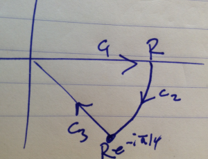
Note that the integral above has value \( \sqrt{-i\pi} \) which can be found by integrating over the contour of fig. 1, letting \( R \rightarrow \infty \).

contourFig1

fig. 1. Integration contour for \( \int e^{-i z^2} \)

Multiplying out each of the spatial direction factors gives the propagator in its closed form
\begin{equation}\label{eqn:freeParticlePropagator:120}
\boxed{
K(\Bx”, t ; \Bx’, t_0)
= \lr{ \sqrt{ \frac{ m }{ 2 \pi i \Hbar (t -t_0)} } }^3
\exp\lr{ \frac{i(\Bx” – \Bx’)^2 m}{2 (t -t_0) \Hbar} }.
}
\end{equation}

In one or two dimensions the exponential power \( 3 \) need only be adjusted appropriately.

Question: Momentum space free particle propagator ([1] pr. 2.33)

Derive the free particle propagator in momentum space.

Answer

The momentum space propagator follows in the same fashion as the spatial propagator

\begin{equation}\label{eqn:freeParticlePropagator:140}
\begin{aligned}
\braket{\Bp”}{\alpha, t ; t_0 }
&= \bra{\Bp”} U \ket{\alpha, t_0 } \\
&= \bra{\Bp”} e^{-i H (t -t_0)/\Hbar} \ket{\alpha, t_0 } \\
&= \bra{\Bp”} e^{-i H (t -t_0)/\Hbar} \lr{ \sum_{a’} \ket{a’} \bra{a’ }} \ket{\alpha, t_0 } \\
&= \bra{\Bp”} \sum_{a’} e^{-i E_{a’} (t -t_0)/\Hbar} \ket{a’} \braket{a’ }{\alpha, t_0 } \\
&=
\bra{\Bp”} \sum_{a’} e^{-i E_{a’} (t -t_0)/\Hbar} \ket{a’} \bra{a’ }
\lr{ \int d^3 \Bp’
\ket{\Bp’}\bra{\Bp’}
}
\ket{\alpha, t_0 } \\
&=
\int d^3 \Bp’
\lr{
\bra{\Bp”} \sum_{a’} e^{-i E_{a’} (t -t_0)/\Hbar} \ket{a’} \braket{a’ }{\Bp’}
}
\braket{\Bp’}{\alpha, t_0 } \\
&=
\int d^3 \Bp’ K(\Bp”, t ; \Bp’, t_0) \braket{\Bp’}{\alpha, t_0 },
\end{aligned}
\end{equation}

so

\begin{equation}\label{eqn:freeParticlePropagator:160}
K(\Bp”, t ; \Bp’, t_0)
=
\sum_{a’}
\braket{\Bp”}{a’}
\braket{a’ }{\Bp’}
e^{-i E_{a’} (t -t_0)/\Hbar}.
\end{equation}

For the free particle Hamiltonian, this can be evaluated over a momentum space basis

\begin{equation}\label{eqn:freeParticlePropagator:170}
\begin{aligned}
K(\Bp”, t ; \Bp’, t_0)
&=
\int d^3 \Bp”’
\braket{\Bp”}{\Bp”’}
\braket{\Bp”’ }{\Bp’}
e^{-i E_{\Bp”’} (t -t_0)/\Hbar} \\
&=
\int d^3 \Bp”’
\braket{\Bp”}{\Bp”’}
\delta(\Bp”’ – \Bp’)
\exp\lr{ -i \frac{(\Bp”’)^2 (t -t_0)}{2 m \Hbar}} \\
&=
\braket{\Bp”}{\Bp’}
\exp\lr{ -i \frac{(\Bp’)^2 (t -t_0)}{2 m \Hbar}}
\end{aligned}
\end{equation}

or

\begin{equation}\label{eqn:freeParticlePropagator:200}
\boxed{
K(\Bp”, t ; \Bp’, t_0)
=
\delta( \Bp” – \Bp’ )
\exp\lr{ -i \frac{(\Bp’)^2 (t -t_0)}{2 m \Hbar}}.
}
\end{equation}

This is what we expect since the time evolution is given by just this exponential factor

\begin{equation}\label{eqn:freeParticlePropagator:220}
\begin{aligned}
\braket{\Bp’}{\alpha, t_0 ; t}
&= \bra{\Bp’} \exp\lr{ -i \frac{(\Bp’)^2 (t -t_0)}{2 m \Hbar}} \ket{\alpha, t_0} \\
&=
\exp\lr{ -i \frac{(\Bp’)^2 (t -t_0)}{2 m \Hbar}}
\braket{\Bp’}
{\alpha, t_0}.
\end{aligned}
\end{equation}

References

[1] Jun John Sakurai and Jim J Napolitano. Modern quantum mechanics. Pearson Higher Ed, 2014.