[Click here for a PDF of this post with nicer formatting]
A problem posed in the ece1228 problem set was the following
Helmholtz theorem.
Prove the first Helmholtz’s theorem, i.e. if vector \(\BM\) is defined by its divergence
\begin{equation}\label{eqn:emtProblemSet1Problem5:20}
\spacegrad \cdot \BM = s
\end{equation}
and its curl
\begin{equation}\label{eqn:emtProblemSet1Problem5:40}
\spacegrad \cross \BM = \BC
\end{equation}
within a region and its normal component \( \BM_{\textrm{n}} \) over the boundary, then \( \BM \) is uniquely specified.
Solution.
This problem screams for an attempt using Geometric Algebra techniques, since
the gradient of this vector can be written as a single even grade multivector
\begin{equation}\label{eqn:emtProblemSet1Problem5AppendixGA:60}
\begin{aligned}
\spacegrad \BM
&= \spacegrad \cdot \BM + I \spacegrad \cross \BM \\
&= s + I \BC.
\end{aligned}
\end{equation}
Observe that the Laplacian of \( \BM \) is vector valued
\begin{equation}\label{eqn:emtProblemSet1Problem5AppendixGA:400}
\spacegrad^2 \BM
= \spacegrad s + I \spacegrad \BC.
\end{equation}
This means that \( \spacegrad \BC \) must be a bivector \( \spacegrad \BC = \spacegrad \wedge \BC \), or that \( \BC \) has zero divergence
\begin{equation}\label{eqn:emtProblemSet1Problem5AppendixGA:420}
\spacegrad \cdot \BC = 0.
\end{equation}
This required constraint on \( \BC \) will show up in subsequent analysis. An equivalent problem to the one posed
is to show that the even grade multivector equation \( \spacegrad \BM = s + I \BC \) has an inverse given the constraint
specified by \ref{eqn:emtProblemSet1Problem5AppendixGA:420}.
Inverting the gradient equation.
The Green’s function for the gradient can be found in [1], where it is used to generalize the Cauchy integral equations to higher dimensions.
\begin{equation}\label{eqn:emtProblemSet1Problem5AppendixGA:80}
\begin{aligned}
G(\Bx ; \Bx’) &= \inv{4 \pi} \frac{ \Bx – \Bx’ }{\Abs{\Bx – \Bx’}^3} \\
\spacegrad \BG(\Bx, \Bx’) &= \spacegrad \cdot \BG(\Bx, \Bx’) = \delta(\Bx – \Bx’) = -\spacegrad’ \BG(\Bx, \Bx’).
\end{aligned}
\end{equation}
The inversion equation is an application of the Fundamental Theorem of (Geometric) Calculus, with the gradient operating bidirectionally on the Green’s function and the vector function
\begin{equation}\label{eqn:emtProblemSet1Problem5AppendixGA:100}
\begin{aligned}
\oint_{\partial V} G(\Bx, \Bx’) d^2 \Bx’ \BM(\Bx’)
&=
\int_V G(\Bx, \Bx’) d^3 \Bx \lrspacegrad’ \BM(\Bx’) \\
&=
\int_V d^3 \Bx (G(\Bx, \Bx’) \lspacegrad’) \BM(\Bx’)
+
\int_V d^3 \Bx G(\Bx, \Bx’) (\spacegrad’ \BM(\Bx’)) \\
&=
-\int_V d^3 \Bx \delta(\Bx – \By) \BM(\Bx’)
+
\int_V d^3 \Bx G(\Bx, \Bx’) \lr{ s(\Bx’) + I \BC(\Bx’) } \\
&=
-I \BM(\Bx)
+
\inv{4 \pi} \int_V d^3 \Bx \frac{ \Bx – \Bx’}{ \Abs{\Bx – \Bx’}^3 } \lr{ s(\Bx’) + I \BC(\Bx’) }.
\end{aligned}
\end{equation}
The integrals are in terms of the primed coordinates so that the end result is a function of \( \Bx \). To rearrange for \( \BM \), let \( d^3 \Bx’ = I dV’ \), and \( d^2 \Bx’ \ncap(\Bx’) = I dA’ \), then right multiply with the pseudoscalar \( I \), noting that in \R{3} the pseudoscalar commutes with any grades
\begin{equation}\label{eqn:emtProblemSet1Problem5AppendixGA:440}
\begin{aligned}
\BM(\Bx)
&=
I \oint_{\partial V} G(\Bx, \Bx’) I dA’ \ncap \BM(\Bx’)
–
I \inv{4 \pi} \int_V I dV’ \frac{ \Bx – \Bx’}{ \Abs{\Bx – \Bx’}^3 } \lr{ s(\Bx’) + I \BC(\Bx’) } \\
&=
-\oint_{\partial V} dA’ G(\Bx, \Bx’) \ncap \BM(\Bx’)
+
\inv{4 \pi} \int_V dV’ \frac{ \Bx – \Bx’}{ \Abs{\Bx – \Bx’}^3 } \lr{ s(\Bx’) + I \BC(\Bx’) }.
\end{aligned}
\end{equation}
This can be decomposed into a vector and a trivector equation. Let \( \Br = \Bx – \Bx’ = r \rcap \), and note that
\begin{equation}\label{eqn:emtProblemSet1Problem5AppendixGA:500}
\begin{aligned}
\gpgradeone{ \rcap I \BC }
&=
\gpgradeone{ I \rcap \BC } \\
&=
I \rcap \wedge \BC \\
&=
-\rcap \cross \BC,
\end{aligned}
\end{equation}
so this pair of equations can be written as
\begin{equation}\label{eqn:emtProblemSet1Problem5AppendixGA:520}
\begin{aligned}
\BM(\Bx)
&=
-\inv{4 \pi} \oint_{\partial V} dA’ \frac{\gpgradeone{ \rcap \ncap \BM(\Bx’) }}{r^2}
+
\inv{4 \pi} \int_V dV’ \lr{
\frac{\rcap}{r^2} s(\Bx’) –
\frac{\rcap}{r^2} \cross \BC(\Bx’) } \\
0
&=
-\inv{4 \pi} \oint_{\partial V} dA’ \frac{\rcap}{r^2} \wedge \ncap \wedge \BM(\Bx’)
+
\frac{I}{4 \pi} \int_V dV’ \frac{ \rcap \cdot \BC(\Bx’) }{r^2}.
\end{aligned}
\end{equation}
Trivector grades.
Consider the last integral in the pseudoscalar equation above. Since we expect no pseudoscalar components, this must be zero, or cancel perfectly. It’s not obvious that this is the case, but a transformation to a surface integral shows the constraints required for that to be the case. To do so note
\begin{equation}\label{eqn:emtProblemSet1Problem5AppendixGA:540}
\begin{aligned}
\spacegrad \inv{\Bx – \Bx’}
&= -\spacegrad’ \inv{\Bx – \Bx’} \\
&=
-\frac{\Bx – \Bx’}{\Abs{\Bx – \Bx’}^3} \\
&= -\frac{\rcap}{r^2}.
\end{aligned}
\end{equation}
Using this and the chain rule we have
\begin{equation}\label{eqn:emtProblemSet1Problem5AppendixGA:560}
\begin{aligned}
\frac{I}{4 \pi} \int_V dV’ \frac{ \rcap \cdot \BC(\Bx’) }{r^2}
&=
\frac{I}{4 \pi} \int_V dV’ \lr{ \spacegrad’ \inv{ r } } \cdot \BC(\Bx’) \\
&=
\frac{I}{4 \pi} \int_V dV’ \spacegrad’ \cdot \frac{\BC(\Bx’)}{r}
–
\frac{I}{4 \pi} \int_V dV’ \frac{ \spacegrad’ \cdot \BC(\Bx’) }{r} \\
&=
\frac{I}{4 \pi} \int_V dV’ \spacegrad’ \cdot \frac{\BC(\Bx’)}{r} \\
&=
\frac{I}{4 \pi} \int_{\partial V} dA’ \ncap(\Bx’) \cdot \frac{\BC(\Bx’)}{r}.
\end{aligned}
\end{equation}
The divergence of \( \BC \) above was killed by recalling the constraint \ref{eqn:emtProblemSet1Problem5AppendixGA:420}. This means that we can rewrite entirely as surface integral and eventually reduced to a single triple product
\begin{equation}\label{eqn:emtProblemSet1Problem5AppendixGA:580}
\begin{aligned}
0
&=
-\frac{I}{4 \pi} \oint_{\partial V} dA’ \lr{
\frac{\rcap}{r^2} \cdot (\ncap \cross \BM(\Bx’))
-\ncap \cdot \frac{\BC(\Bx’)}{r}
} \\
&=
\frac{I}{4 \pi} \oint_{\partial V} dA’ \ncap \cdot \lr{
\frac{\rcap}{r^2} \cross \BM(\Bx’)
+ \frac{\BC(\Bx’)}{r}
} \\
&=
\frac{I}{4 \pi} \oint_{\partial V} dA’ \ncap \cdot \lr{
\lr{ \spacegrad’ \inv{r}} \cross \BM(\Bx’)
+ \frac{\BC(\Bx’)}{r}
} \\
&=
\frac{I}{4 \pi} \oint_{\partial V} dA’ \ncap \cdot \lr{
\spacegrad’ \cross \frac{\BM(\Bx’)}{r}
} \\
&=
\frac{I}{4 \pi} \oint_{\partial V} dA’
\spacegrad’ \cdot
\frac{\BM(\Bx’) \cross \ncap}{r}
&=
\frac{I}{4 \pi} \oint_{\partial V} dA’
\spacegrad’ \cdot
\frac{\BM(\Bx’) \cross \ncap}{r}.
\end{aligned}
\end{equation}
Final results.
Assembling things back into a single multivector equation, the complete inversion integral for \( \BM \) is
\begin{equation}\label{eqn:emtProblemSet1Problem5AppendixGA:600}
\BM(\Bx)
=
\inv{4 \pi} \oint_{\partial V} dA’
\lr{
\spacegrad’ \wedge
\frac{\BM(\Bx’) \wedge \ncap}{r}
-\frac{\gpgradeone{ \rcap \ncap \BM(\Bx’) }}{r^2}
}
+
\inv{4 \pi} \int_V dV’ \lr{
\frac{\rcap}{r^2} s(\Bx’) –
\frac{\rcap}{r^2} \cross \BC(\Bx’) }.
\end{equation}
This shows that vector \( \BM \) can be recovered uniquely from \( s, \BC \) when \( \Abs{\BM}/r^2 \) vanishes on an infinite surface. If we restrict attention to a finite surface, we have to add to the fixed solution a specific solution that depends on the value of \( \BM \) on that surface. The vector portion of that surface integrand contains
\begin{equation}\label{eqn:emtProblemSet1Problem5AppendixGA:640}
\begin{aligned}
\gpgradeone{ \rcap \ncap \BM }
&=
\rcap (\ncap \cdot \BM )
+
\rcap \cdot (\ncap \wedge \BM ) \\
&=
\rcap (\ncap \cdot \BM )
+
(\rcap \cdot \ncap) \BM
–
(\rcap \cdot \BM ) \ncap.
\end{aligned}
\end{equation}
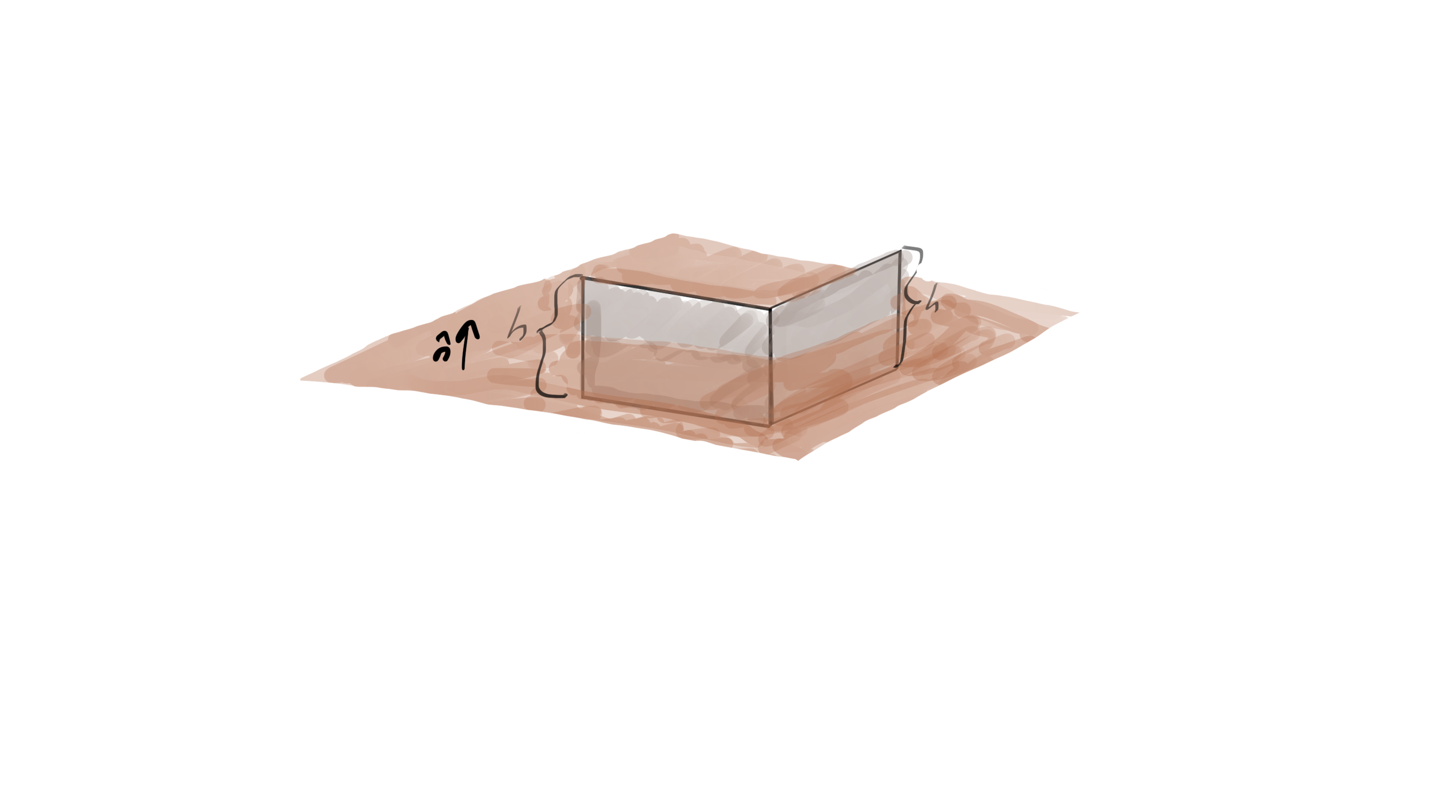
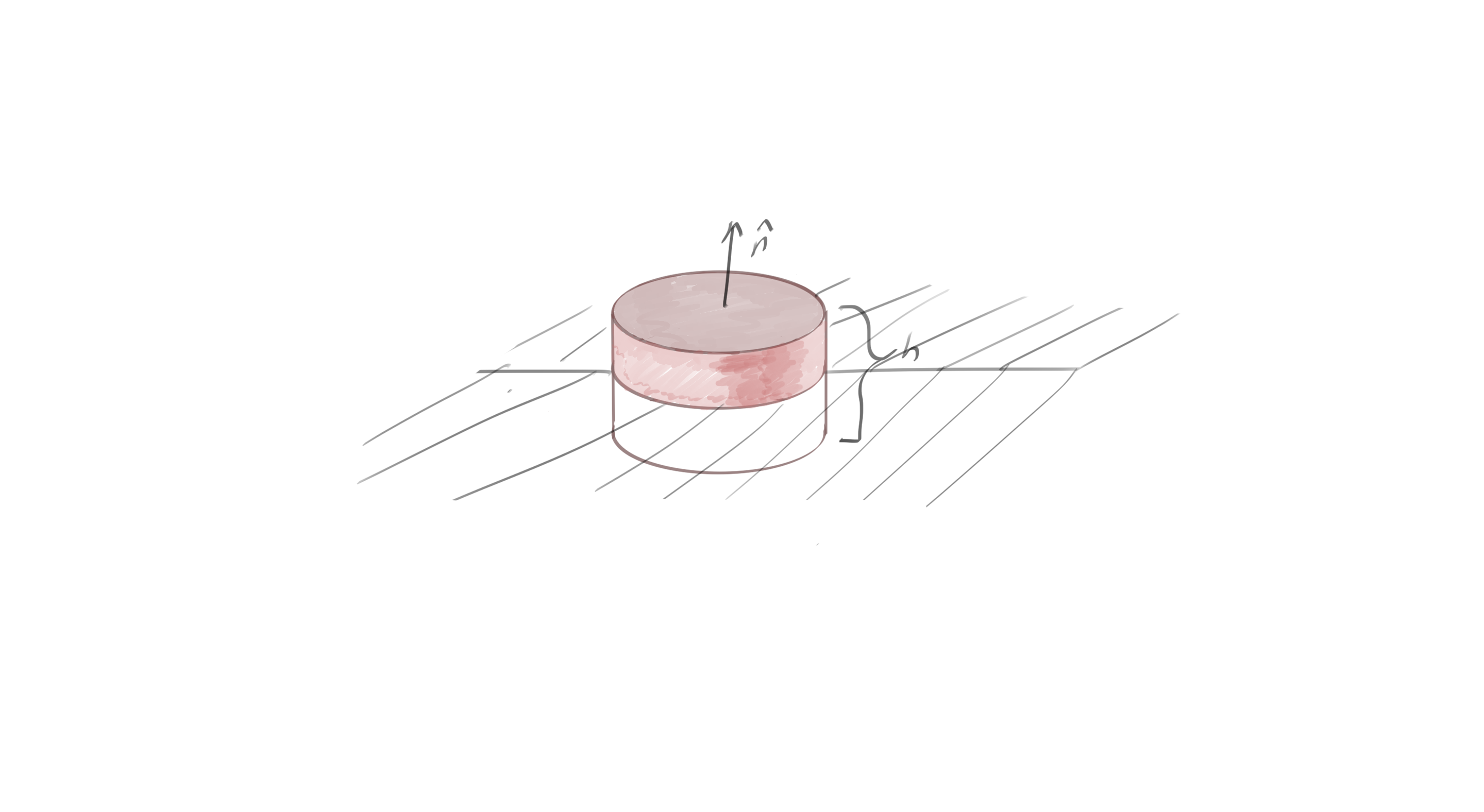
The constraints required by a zero triple product \( \spacegrad’ \cdot (\BM(\Bx’) \cross \ncap(\Bx’)) \) are complicated on a such a general finite surface. Consider instead, for simplicity, the case of a spherical surface, which can be analyzed more easily. In that case the outward normal of the surface centred on the test charge point \( \Bx \) is \( \ncap = -\rcap \). The pseudoscalar integrand is not generally killed unless the divergence of its tangential component on this surface is zero. One way that this can occur is for \( \BM \cross \ncap = 0 \), so that \( -\gpgradeone{ \rcap \ncap \BM } = \BM = (\BM \cdot \ncap) \ncap = \BM_{\textrm{n}} \).
This gives
\begin{equation}\label{eqn:emtProblemSet1Problem5AppendixGA:620}
\BM(\Bx)
=
\inv{4 \pi} \oint_{\Abs{\Bx – \Bx’} = r} dA’ \frac{\BM_{\textrm{n}}(\Bx’)}{r^2}
+
\inv{4 \pi} \int_V dV’ \lr{
\frac{\rcap}{r^2} s(\Bx’) +
\BC(\Bx’) \cross \frac{\rcap}{r^2} },
\end{equation}
or, in terms of potential functions, which is arguably tidier
\begin{equation}\label{eqn:emtProblemSet1Problem5AppendixGA:300}
\boxed{
\BM(\Bx)
=
\inv{4 \pi} \oint_{\Abs{\Bx – \Bx’} = r} dA’ \frac{\BM_{\textrm{n}}(\Bx’)}{r^2}
-\spacegrad \int_V dV’ \frac{ s(\Bx’)}{ 4 \pi r }
+\spacegrad \cross \int_V dV’ \frac{ \BC(\Bx’) }{ 4 \pi r }.
}
\end{equation}
Commentary
I attempted this problem in three different ways. My first approach (above) assembled the divergence and curl relations above into a single (Geometric Algebra) multivector gradient equation and applied the vector valued Green’s function for the gradient to invert that equation. That approach logically led from the differential equation for \( \BM \) to the solution for \( \BM \) in terms of \( s \) and \( \BC \). However, this strategy introduced some complexities that make me doubt the correctness of the associated boundary analysis.
Even if the details of the boundary handling in my multivector approach is not correct, I thought that approach was interesting enough to share.
References
[1] C. Doran and A.N. Lasenby. Geometric algebra for physicists. Cambridge University Press New York, Cambridge, UK, 1st edition, 2003.