Maxwell’s equation

Some nice positive feedback for my book.

October 31, 2020 math and physics play , , , , , , , , , ,

Here’s a fun congratulatory email that I received today for my Geometric Algebra for Electrical Engineers book

Peeter ..
I had to email to congratulate you on your geometric algebra book. Like yourself, when I came across it, I was totally blown away and your book, being written from the position of a discoverer rather than an expert, answers most of the questions I was confronted by when reading Doran and Lasenby’s book.
You’re a C++ programmer and from my perspective, when using natural world math, you are constructing a representation of a problem (like code does) except many physicists do not recognize this. They’re doing physics with COBOL (or C with classes!).
congratulations
.. Reader
I couldn’t resist pointing out the irony of his COBOL comment, as my work at LzLabs is now heavily focused on COBOL (and PL/I) compilers and compiler runtimes.  You could say that my work, at work or at play, is all an attempt to transition people away from the evils of legacy COBOL.
For reference the Doran and Lasenby book is phenomenal work, but it is really hard material.  To attempt to read this, you’ll need a thorough understanding of electromagnetism, relativity, tensor algebra, quantum mechanics, advanced classical mechanics, and field theory.  I’m still working on this book, and it’s probably been 12 years since I bought it.  I managed to teach myself some of this material as I went, but also took most of the 4th year UofT undergrad physics courses (and some grad courses) to fill in some of the gaps.
When I titled my book, I included “for Electrical Engineers” in the title.  That titling choice was somewhat derivative, as there were already geometric algebra books “for physicists”,  and “for computer science“.  However, I thought it was also good shorthand for the prerequisites required for the book as “for Electrical Engineers” seemed to be good shorthand for “for a student that has seen electromagnetism in its div, grad, curl form, and doesn’t know special relativity, field theory, differential forms, tensor algebra, or other topics from more advanced physics.”
The relativistic presentation of electromagnetism in Doran and Lasenby, using the Dirac algebra (aka Space Time Algebra (STA)), is much more beautiful than the form that I have used in my book.  However, I was hoping to present the subject in a way that was accessible, and provided a stepping stone for the STA approach when the reader was ready to tackle a next interval of the “learning curve.”

Applied vanity press

April 9, 2018 math and physics play , , , ,

Amazon’s createspace turns out to be a very cost effective way to get a personal color copy of large pdf (>250 pages) to markup for review. The only hassle was having to use their app to create cover art (although that took less time than commuting downtown to one of the cheap copy shops near the university.)

As a side effect, after I edit it, I’d have something I could actually list for sale.  Worldwide, I’d guess at least three people would buy it, that is, if they weren’t happy with the pdf version already available.

I wrote a book: Geometric Algebra for Electrical Engineers

April 5, 2018 math and physics play , ,

The book.

A draft of my book: Geometric Algebra for Electrical Engineers, is now available. I’ve supplied limited distribution copies of some of the early drafts and have had some good review comments of the chapter I (introduction to geometric algebra), and chapter II (multivector calculus) material, but none on the electromagnetism content. In defense of the reviewers, the initial version of the electromagnetism chapter, while it had a lot of raw content, was pretty exploratory and very rough. It’s been cleaned up significantly and is hopefully now more reader friendly.

Why I wrote this book.

I have been working on a part time M.Eng degree for a number of years. I wasn’t happy with the UofT ECE electromagnetics offerings in recent years, which have been inconsistently offered or unsatisfactory. For example: the microwave circuits course which sounded interesting, and had an interesting text book, was mind numbing, almost entirely about Smith charts. I had to go elsewhere to obtain the M.Eng degree requirements. That elsewhere was a project course.

I proposed a project to an electromagnetism project with the following goals

  1. Perform a literature review of applications of geometric algebra to the study of electromagnetism.
  2. Identify the subset of the literature that had direct relevance to electrical engineering.
  3. Create a complete, and as compact as possible, introduction to the prerequisites required for a graduate or advanced undergraduate electrical engineering student to be able to apply geometric algebra to problems in electromagnetism. With those prerequisites in place, work through the fundamentals of electromagnetism in a geometric algebra context.

In retrospect, doing this project was a mistake. I could have done this work outside of an academic context without paying so much (in both time and money). Somewhere along the way I lost track of the fact that I enrolled on the M.Eng to learn (it provided a way to take grad physics courses on a part time schedule), and got side tracked by degree requirements. Basically I fell victim to a “I may as well graduate” sentiment that would have been better to ignore. All that coupled with the fact that I did not actually get any feedback from my “supervisor”, who did not even read my work (at least so far after one year), made this project-course very frustrating. On the bright side, I really like what I produced, even if I had to do so in isolation.

Why geometric algebra?

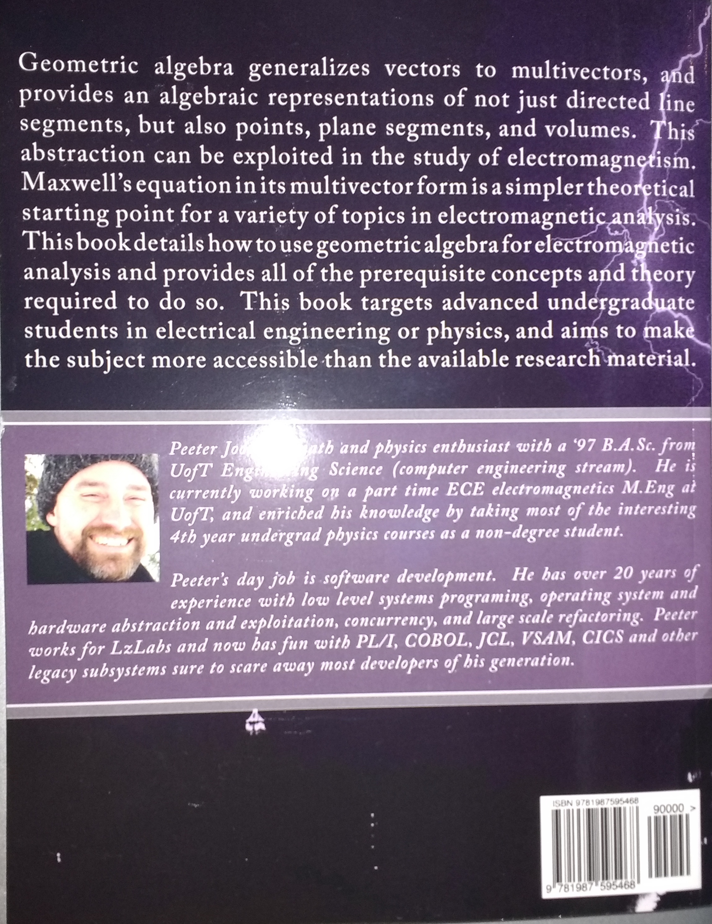
Geometric algebra generalizes vectors, providing algebraic representations of not just directed line segments, but also points, plane segments, volumes, and higher degree geometric objects (hypervolumes.). The geometric algebra representation of planes, volumes and hypervolumes requires a vector dot product, a vector multiplication operation, and a generalized addition operation. The dot product provides the length of a vector and a test for whether or not any two vectors are perpendicular. The vector multiplication operation is used to construct directed plane segments (bivectors), and directed volumes (trivectors), which are built from the respective products of two or three mutually perpendicular vectors. The addition operation allows for sums of scalars, vectors, or any products of vectors. Such a sum is called a multivector.

The power to add scalars, vectors, and products of vectors can be exploited to simplify much of electromagnetism. In particular, Maxwell’s equations for isotropic media can be merged into a single multivector equation
\begin{equation}\label{eqn:quaternion2maxwellWithGA:20}
\lr{ \spacegrad + \inv{c} \PD{t}{}} \lr{ \BE + I c \BB } = \eta\lr{ c \rho – \BJ },
\end{equation}
where \( \spacegrad \) is the gradient, \( I = \Be_1 \Be_2 \Be_3 \) is the ordered product of the three R^3 basis vectors, \( c = 1/\sqrt{\mu\epsilon}\) is the group velocity of the medium, \( \eta = \sqrt{\mu/\epsilon} \), \( \BE, \BB \) are the electric and magnetic fields, and \( \rho \) and \( \BJ \) are the charge and current densities. This can be written as a single equation
\begin{equation}\label{eqn:ece2500report:40}
\lr{ \spacegrad + \inv{c} \PD{t}{}} F = J,
\end{equation}
where \( F = \BE + I c \BB \) is the combined (multivector) electromagnetic field, and \( J = \eta\lr{ c \rho – \BJ } \) is the multivector current.

Encountering Maxwell’s equation in its geometric algebra form leaves the student with more questions than answers. Yes, it is a compact representation, but so are the tensor and differential forms (or even the quaternionic) representations of Maxwell’s equations. The student needs to know how to work with the representation if it is to be useful. It should also be clear how to use the existing conventional mathematical tools of applied electromagnetism, or how to generalize those appropriately. Individually, there are answers available to many of the questions that are generated attempting to apply the theory, but they are scattered and in many cases not easily accessible.

Much of the geometric algebra literature for electrodynamics is presented with a relativistic bias, or assumes high levels of mathematical or physics sophistication. The aim of this work was an attempt to make the study of electromagnetism using geometric algebra more accessible, especially to other dumb engineering undergraduates like myself. In particular, this project explored non-relativistic applications of geometric algebra to electromagnetism. The end product of this project was a fairly small self contained book, titled “Geometric Algebra for Electrical Engineers”. This book includes an introduction to Euclidean geometric algebra focused on R^2 and R^3 (64 pages), an introduction to geometric calculus and multivector Green’s functions (64 pages), applications to electromagnetism (82 pages), and some appendices. Many of the fundamental results of electromagnetism are derived directly from the multivector Maxwell’s equation, in a streamlined and compact fashion. This includes some new results, and many of the existing non-relativistic results from the geometric algebra literature. As a conceptual bridge, the book includes many examples of how to extract familiar conventional results from simpler multivector representations. Also included in the book are some sample calculations exploiting unique capabilities that geometric algebra provides. In particular, vectors in a plane may be manipulated much like complex numbers, which has a number of advantages over working with coordinates explicitly.

Followup.

In many ways this work only scratches the surface. Many more worked examples, problems, figures and computer algebra listings should be added. In depth applications of derived geometric algebra relationships to problems customarily tackled with separate electric and magnetic field equations should also be incorporated. There are also theoretical holes, topics covered in any conventional introductory electromagnetism text, that are missing. Examples include the Fresnel relationships for transmission and reflection at an interface, in depth treatment of waveguides, dipole radiation and motion of charged particles, bound charges, and meta materials to name a few. Many of these topics can probably be handled in a coordinate free fashion using geometric algebra. Despite all the work that is required to help bridge the gap between formalism and application, making applied electromagnetism using geometric algebra truly accessible, it is my belief this book makes some good first steps down this path.

The choice that I made to completely avoid the geometric algebra space-time-algebra (STA) is somewhat unfortunate. It is exceedingly elegant, especially in a relativisitic context. Despite that, I think that this was still a good choice from a pedagogical point of view, as most of the prerequisites for an STA based study will have been taken care of as a side effect, making that study much more accessible.

Potential solutions to the static Maxwell’s equation using geometric algebra

March 20, 2018 math and physics play , , , , , , , , , , , , , , , , ,

[Click here for a PDF of this post with nicer formatting]

When neither the electromagnetic field strength \( F = \BE + I \eta \BH \), nor current \( J = \eta (c \rho – \BJ) + I(c\rho_m – \BM) \) is a function of time, then the geometric algebra form of Maxwell’s equations is the first order multivector (gradient) equation
\begin{equation}\label{eqn:staticPotentials:20}
\spacegrad F = J.
\end{equation}

While direct solutions to this equations are possible with the multivector Green’s function for the gradient
\begin{equation}\label{eqn:staticPotentials:40}
G(\Bx, \Bx’) = \inv{4\pi} \frac{\Bx – \Bx’}{\Norm{\Bx – \Bx’}^3 },
\end{equation}
the aim in this post is to explore second order (potential) solutions in a geometric algebra context. Can we assume that it is possible to find a multivector potential \( A \) for which
\begin{equation}\label{eqn:staticPotentials:60}
F = \spacegrad A,
\end{equation}
is a solution to the Maxwell statics equation? If such a solution exists, then Maxwell’s equation is simply
\begin{equation}\label{eqn:staticPotentials:80}
\spacegrad^2 A = J,
\end{equation}
which can be easily solved using the scalar Green’s function for the Laplacian
\begin{equation}\label{eqn:staticPotentials:240}
G(\Bx, \Bx’) = -\inv{\Norm{\Bx – \Bx’} },
\end{equation}
a beastie that may be easier to convolve than the vector valued Green’s function for the gradient.

It is immediately clear that some restrictions must be imposed on the multivector potential \(A\). In particular, since the field \( F \) has only vector and bivector grades, this gradient must have no scalar, nor pseudoscalar grades. That is
\begin{equation}\label{eqn:staticPotentials:100}
\gpgrade{\spacegrad A}{0,3} = 0.
\end{equation}
This constraint on the potential can be avoided if a grade selection operation is built directly into the assumed potential solution, requiring that the field is given by
\begin{equation}\label{eqn:staticPotentials:120}
F = \gpgrade{\spacegrad A}{1,2}.
\end{equation}
However, after imposing such a constraint, Maxwell’s equation has a much less friendly form
\begin{equation}\label{eqn:staticPotentials:140}
\spacegrad^2 A – \spacegrad \gpgrade{\spacegrad A}{0,3} = J.
\end{equation}
Luckily, it is possible to introduce a transformation of potentials, called a gauge transformation, that eliminates the ugly grade selection term, and allows the potential equation to be expressed as a plain old Laplacian. We do so by assuming first that it is possible to find a solution of the Laplacian equation that has the desired grade restrictions. That is
\begin{equation}\label{eqn:staticPotentials:160}
\begin{aligned}
\spacegrad^2 A’ &= J \\
\gpgrade{\spacegrad A’}{0,3} &= 0,
\end{aligned}
\end{equation}
for which \( F = \spacegrad A’ \) is a grade 1,2 solution to \( \spacegrad F = J \). Suppose that \( A \) is any formal solution, free of any grade restrictions, to \( \spacegrad^2 A = J \), and \( F = \gpgrade{\spacegrad A}{1,2} \). Can we find a function \( \tilde{A} \) for which \( A = A’ + \tilde{A} \)?

Maxwell’s equation in terms of \( A \) is
\begin{equation}\label{eqn:staticPotentials:180}
\begin{aligned}
J
&= \spacegrad \gpgrade{\spacegrad A}{1,2} \\
&= \spacegrad^2 A
– \spacegrad \gpgrade{\spacegrad A}{0,3} \\
&= \spacegrad^2 (A’ + \tilde{A})
– \spacegrad \gpgrade{\spacegrad A}{0,3}
\end{aligned}
\end{equation}
or
\begin{equation}\label{eqn:staticPotentials:200}
\spacegrad^2 \tilde{A} = \spacegrad \gpgrade{\spacegrad A}{0,3}.
\end{equation}
This non-homogeneous Laplacian equation that can be solved as is for \( \tilde{A} \) using the Green’s function for the Laplacian. Alternatively, we may also solve the equivalent first order system using the Green’s function for the gradient.
\begin{equation}\label{eqn:staticPotentials:220}
\spacegrad \tilde{A} = \gpgrade{\spacegrad A}{0,3}.
\end{equation}
Clearly \( \tilde{A} \) is not unique, as we can add any function \( \psi \) satisfying the homogeneous Laplacian equation \( \spacegrad^2 \psi = 0 \).

In summary, if \( A \) is any multivector solution to \( \spacegrad^2 A = J \), that is
\begin{equation}\label{eqn:staticPotentials:260}
A(\Bx)
= \int dV’ G(\Bx, \Bx’) J(\Bx’)
= -\int dV’ \frac{J(\Bx’)}{\Norm{\Bx – \Bx’} },
\end{equation}
then \( F = \spacegrad A’ \) is a solution to Maxwell’s equation, where \( A’ = A – \tilde{A} \), and \( \tilde{A} \) is a solution to the non-homogeneous Laplacian equation or the non-homogeneous gradient equation above.

Integral form of the gauge transformation.

Additional insight is possible by considering the gauge transformation in integral form. Suppose that
\begin{equation}\label{eqn:staticPotentials:280}
A(\Bx) = -\int_V dV’ \frac{J(\Bx’)}{\Norm{\Bx – \Bx’} } – \tilde{A}(\Bx),
\end{equation}
is a solution of \( \spacegrad^2 A = J \), where \( \tilde{A} \) is a multivector solution to the homogeneous Laplacian equation \( \spacegrad^2 \tilde{A} = 0 \). Let’s look at the constraints on \( \tilde{A} \) that must be imposed for \( F = \spacegrad A \) to be a valid (i.e. grade 1,2) solution of Maxwell’s equation.
\begin{equation}\label{eqn:staticPotentials:300}
\begin{aligned}
F
&= \spacegrad A \\
&=
-\int_V dV’ \lr{ \spacegrad \inv{\Norm{\Bx – \Bx’} } } J(\Bx’)
– \spacegrad \tilde{A}(\Bx) \\
&=
\int_V dV’ \lr{ \spacegrad’ \inv{\Norm{\Bx – \Bx’} } } J(\Bx’)
– \spacegrad \tilde{A}(\Bx) \\
&=
\int_V dV’ \spacegrad’ \frac{J(\Bx’)}{\Norm{\Bx – \Bx’} } – \int_V dV’ \frac{\spacegrad’ J(\Bx’)}{\Norm{\Bx – \Bx’} }
– \spacegrad \tilde{A}(\Bx) \\
&=
\int_{\partial V} dA’ \ncap’ \frac{J(\Bx’)}{\Norm{\Bx – \Bx’} } – \int_V \frac{\spacegrad’ J(\Bx’)}{\Norm{\Bx – \Bx’} }
– \spacegrad \tilde{A}(\Bx).
\end{aligned}
\end{equation}
Where \( \ncap’ = (\Bx’ – \Bx)/\Norm{\Bx’ – \Bx} \), and the fundamental theorem of geometric calculus has been used to transform the gradient volume integral into an integral over the bounding surface. Operating on Maxwell’s equation with the gradient gives \( \spacegrad^2 F = \spacegrad J \), which has only grades 1,2 on the left hand side, meaning that \( J \) is constrained in a way that requires \( \spacegrad J \) to have only grades 1,2. This means that \( F \) has grades 1,2 if
\begin{equation}\label{eqn:staticPotentials:320}
\spacegrad \tilde{A}(\Bx)
= \int_{\partial V} dA’ \frac{ \gpgrade{\ncap’ J(\Bx’)}{0,3} }{\Norm{\Bx – \Bx’} }.
\end{equation}
The product \( \ncap J \) expands to
\begin{equation}\label{eqn:staticPotentials:340}
\begin{aligned}
\ncap J
&=
\gpgradezero{\ncap J_1} + \gpgradethree{\ncap J_2} \\
&=
\ncap \cdot (-\eta \BJ) + \gpgradethree{\ncap (-I \BM)} \\
&=- \eta \ncap \cdot \BJ -I \ncap \cdot \BM,
\end{aligned}
\end{equation}
so
\begin{equation}\label{eqn:staticPotentials:360}
\spacegrad \tilde{A}(\Bx)
=
-\int_{\partial V} dA’ \frac{ \eta \ncap’ \cdot \BJ(\Bx’) + I \ncap’ \cdot \BM(\Bx’)}{\Norm{\Bx – \Bx’} }.
\end{equation}
Observe that if there is no flux of current density \( \BJ \) and (fictitious) magnetic current density \( \BM \) through the surface, then \( F = \spacegrad A \) is a solution to Maxwell’s equation without any gauge transformation. Alternatively \( F = \spacegrad A \) is also a solution if \( \lim_{\Bx’ \rightarrow \infty} \BJ(\Bx’)/\Norm{\Bx – \Bx’} = \lim_{\Bx’ \rightarrow \infty} \BM(\Bx’)/\Norm{\Bx – \Bx’} = 0 \) and the bounding volume is taken to infinity.

References

Solving Maxwell’s equation in freespace: Multivector plane wave representation

March 14, 2018 math and physics play , , , , , , , , , , , ,

[Click here for a PDF of this post with nicer formatting]

The geometric algebra form of Maxwell’s equations in free space (or source free isotopic media with group velocity \( c \)) is the multivector equation
\begin{equation}\label{eqn:planewavesMultivector:20}
\lr{ \spacegrad + \inv{c}\PD{t}{} } F(\Bx, t) = 0.
\end{equation}
Here \( F = \BE + I c \BB \) is a multivector with grades 1 and 2 (vector and bivector components). The velocity \( c \) is called the group velocity since \( F \), or its components \( \BE, \BH \) satisfy the wave equation, which can be seen by pre-multiplying with \( \spacegrad – (1/c)\PDi{t}{} \) to find
\begin{equation}\label{eqn:planewavesMultivector:n}
\lr{ \spacegrad^2 – \inv{c^2}\PDSq{t}{} } F(\Bx, t) = 0.
\end{equation}

Let’s look at the frequency domain solution of this equation with a presumed phasor representation
\begin{equation}\label{eqn:planewavesMultivector:40}
F(\Bx, t) = \textrm{Re} \lr{ F(\Bk) e^{-j \Bk \cdot \Bx + j \omega t} },
\end{equation}
where \( j \) is a scalar imaginary, not necessarily with any geometric interpretation.

Maxwell’s equation reduces to just
\begin{equation}\label{eqn:planewavesMultivector:60}
0
=
-j \lr{ \Bk – \frac{\omega}{c} } F(\Bk).
\end{equation}

If \( F(\Bk) \) has a left multivector factor
\begin{equation}\label{eqn:planewavesMultivector:80}
F(\Bk) =
\lr{ \Bk + \frac{\omega}{c} } \tilde{F},
\end{equation}
where \( \tilde{F} \) is a multivector to be determined, then
\begin{equation}\label{eqn:planewavesMultivector:100}
\begin{aligned}
\lr{ \Bk – \frac{\omega}{c} }
F(\Bk)
&=
\lr{ \Bk – \frac{\omega}{c} }
\lr{ \Bk + \frac{\omega}{c} } \tilde{F} \\
&=
\lr{ \Bk^2 – \lr{\frac{\omega}{c}}^2 } \tilde{F},
\end{aligned}
\end{equation}
which is zero if \( \Norm{\Bk} = \ifrac{\omega}{c} \).

Let \( \kcap = \ifrac{\Bk}{\Norm{\Bk}} \), and \( \Norm{\Bk} \tilde{F} = F_0 + F_1 + F_2 + F_3 \), where \( F_0, F_1, F_2, \) and \( F_3 \) are respectively have grades 0,1,2,3. Then
\begin{equation}\label{eqn:planewavesMultivector:120}
\begin{aligned}
F(\Bk)
&= \lr{ 1 + \kcap } \lr{ F_0 + F_1 + F_2 + F_3 } \\
&=
F_0 + F_1 + F_2 + F_3
+
\kcap F_0 + \kcap F_1 + \kcap F_2 + \kcap F_3 \\
&=
F_0 + F_1 + F_2 + F_3
+
\kcap F_0 + \kcap \cdot F_1 + \kcap \cdot F_2 + \kcap \cdot F_3
+
\kcap \wedge F_1 + \kcap \wedge F_2 \\
&=
\lr{
F_0 + \kcap \cdot F_1
}
+
\lr{
F_1 + \kcap F_0 + \kcap \cdot F_2
}
+
\lr{
F_2 + \kcap \cdot F_3 + \kcap \wedge F_1
}
+
\lr{
F_3 + \kcap \wedge F_2
}.
\end{aligned}
\end{equation}
Since the field \( F \) has only vector and bivector grades, the grades zero and three components of the expansion above must be zero, or
\begin{equation}\label{eqn:planewavesMultivector:140}
\begin{aligned}
F_0 &= – \kcap \cdot F_1 \\
F_3 &= – \kcap \wedge F_2,
\end{aligned}
\end{equation}
so
\begin{equation}\label{eqn:planewavesMultivector:160}
\begin{aligned}
F(\Bk)
&=
\lr{ 1 + \kcap } \lr{
F_1 – \kcap \cdot F_1 +
F_2 – \kcap \wedge F_2
} \\
&=
\lr{ 1 + \kcap } \lr{
F_1 – \kcap F_1 + \kcap \wedge F_1 +
F_2 – \kcap F_2 + \kcap \cdot F_2
}.
\end{aligned}
\end{equation}
The multivector \( 1 + \kcap \) has the projective property of gobbling any leading factors of \( \kcap \)
\begin{equation}\label{eqn:planewavesMultivector:180}
\begin{aligned}
(1 + \kcap)\kcap
&= \kcap + 1 \\
&= 1 + \kcap,
\end{aligned}
\end{equation}
so for \( F_i \in F_1, F_2 \)
\begin{equation}\label{eqn:planewavesMultivector:200}
(1 + \kcap) ( F_i – \kcap F_i )
=
(1 + \kcap) ( F_i – F_i )
= 0,
\end{equation}
leaving
\begin{equation}\label{eqn:planewavesMultivector:220}
F(\Bk)
=
\lr{ 1 + \kcap } \lr{
\kcap \cdot F_2 +
\kcap \wedge F_1
}.
\end{equation}

For \( \kcap \cdot F_2 \) to be non-zero \( F_2 \) must be a bivector that lies in a plane containing \( \kcap \), and \( \kcap \cdot F_2 \) is a vector in that plane that is perpendicular to \( \kcap \). On the other hand \( \kcap \wedge F_1 \) is non-zero only if \( F_1 \) has a non-zero component that does not lie in along the \( \kcap \) direction, but \( \kcap \wedge F_1 \), like \( F_2 \) describes a plane that containing \( \kcap \). This means that having both bivector and vector free variables \( F_2 \) and \( F_1 \) provide more degrees of freedom than required. For example, if \( \BE \) is any vector, and \( F_2 = \kcap \wedge \BE \), then
\begin{equation}\label{eqn:planewavesMultivector:240}
\begin{aligned}
\lr{ 1 + \kcap }
\kcap \cdot F_2
&=
\lr{ 1 + \kcap }
\kcap \cdot \lr{ \kcap \wedge \BE } \\
&=
\lr{ 1 + \kcap }
\lr{
\BE

\kcap \lr{ \kcap \cdot \BE }
} \\
&=
\lr{ 1 + \kcap }
\kcap \lr{ \kcap \wedge \BE } \\
&=
\lr{ 1 + \kcap }
\kcap \wedge \BE,
\end{aligned}
\end{equation}
which has the form \( \lr{ 1 + \kcap } \lr{ \kcap \wedge F_1 } \), so the solution of the free space Maxwell’s equation can be written
\begin{equation}\label{eqn:planewavesMultivector:260}
\boxed{
F(\Bx, t)
=
\textrm{Re} \lr{
\lr{ 1 + \kcap }
\BE\,
e^{-j \Bk \cdot \Bx + j \omega t}
}
,
}
\end{equation}
where \( \BE \) is any vector for which \( \BE \cdot \Bk = 0 \).