math and physics play

Line charge field and potential.

October 26, 2016 math and physics play , , , , , , , , , ,

[Click here for a PDF of this post with nicer formatting]

When computing the most general solution of the electrostatic potential in a plane, Jackson [1] mentions that \( -2 \lambda_0 \ln \rho \) is the well known potential for an infinite line charge (up to the unit specific factor). Checking that statement, since I didn’t recall what that potential was offhand, I encountered some inconsistencies and non-convergent integrals, and thought it was worthwhile to explore those a bit more carefully. This will be done here.

Using Gauss’s law.

For an infinite length line charge, we can find the radial field contribution using Gauss’s law, imagining a cylinder of length \( \Delta l \) of radius \( \rho \) surrounding this charge with the midpoint at the origin. Ignoring any non-radial field contribution, we have

\begin{equation}\label{eqn:lineCharge:20}
\int_{-\Delta l/2}^{\Delta l/2} \ncap \cdot \BE (2 \pi \rho) dl = \frac{\lambda_0}{\epsilon_0} \Delta l,
\end{equation}

or

\begin{equation}\label{eqn:lineCharge:40}
\BE = \frac{\lambda_0}{2 \pi \epsilon_0} \frac{\rhocap}{\rho}.
\end{equation}

Since

\begin{equation}\label{eqn:lineCharge:60}
\frac{\rhocap}{\rho} = \spacegrad \ln \rho,
\end{equation}

this means that the potential is

\begin{equation}\label{eqn:lineCharge:80}
\phi = -\frac{2 \lambda_0}{4 \pi \epsilon_0} \ln \rho.
\end{equation}

Finite line charge potential.

Let’s try both these calculations for a finite charge distribution. Gauss’s law looses its usefulness, but we can evaluate the integrals directly. For the electric field

\begin{equation}\label{eqn:lineCharge:100}
\BE
= \frac{\lambda_0}{4 \pi \epsilon_0} \int \frac{(\Bx – \Bx’)}{\Abs{\Bx – \Bx’}^3} dl’.
\end{equation}

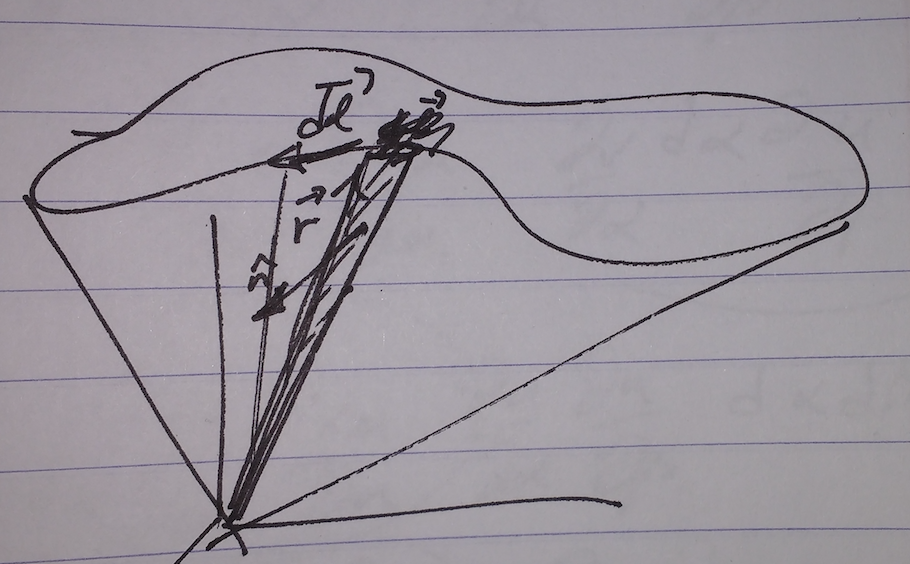
Using cylindrical coordinates with the field point \( \Bx = \rho \rhocap \) for convience, the charge point \( \Bx’ = z’ \zcap \), and a the charge distributed over \( [a,b] \) this is

\begin{equation}\label{eqn:lineCharge:120}
\BE
= \frac{\lambda_0}{4 \pi \epsilon_0} \int_a^b \frac{(\rho \rhocap – z’ \zcap)}{\lr{\rho^2 + (z’)^2}^{3/2}} dz’.
\end{equation}

When the charge is uniformly distributed around the origin \( [a,b] = b[-1,1] \) the \( \zcap \) component of this field is killed because the integrand is odd. This justifies ignoring such contributions in the Gaussing cylinder analysis above. The general solution to this integral is found to be

\begin{equation}\label{eqn:lineCharge:140}
\BE
=
\frac{\lambda_0}{4 \pi \epsilon_0}
\evalrange{
\lr{
\frac{z’ \rhocap }{\rho \sqrt{ \rho^2 + (z’)^2 } }
+\frac{\zcap}{ \sqrt{ \rho^2 + (z’)^2 } }
}
}{a}{b},
\end{equation}

or
\begin{equation}\label{eqn:lineCharge:240}
\boxed{
\BE
=
\frac{\lambda_0}{4 \pi \epsilon_0}
\lr{
\frac{\rhocap }{\rho}
\lr{
\frac{b}{\sqrt{ \rho^2 + b^2 } }
-\frac{a}{\sqrt{ \rho^2 + a^2 } }
}
+ \zcap
\lr{
\frac{1}{ \sqrt{ \rho^2 + b^2 } }
-\frac{1}{ \sqrt{ \rho^2 + a^2 } }
}
}.
}
\end{equation}

When \( b = -a = \Delta l/2 \), this reduces to

\begin{equation}\label{eqn:lineCharge:160}
\BE
=
\frac{\lambda_0}{4 \pi \epsilon_0}
\frac{\rhocap }{\rho}
\frac{\Delta l}{\sqrt{ \rho^2 + (\Delta l/2)^2 } },
\end{equation}

which further reduces to \ref{eqn:lineCharge:40} when \( \Delta l \gg \rho \).

Finite line charge potential. Wrong but illuminating.

Again, putting the field point at \( z’ = 0 \), we have

\begin{equation}\label{eqn:lineCharge:180}
\phi(\rho)
= \frac{\lambda_0}{4 \pi \epsilon_0} \int_a^b \frac{dz’}{\lr{\rho^2 + (z’)^2}^{1/2}},
\end{equation}

which integrates to
\begin{equation}\label{eqn:lineCharge:260}
\phi(\rho)
= \frac{\lambda_0}{4 \pi \epsilon_0 }
\ln \frac{ b + \sqrt{ \rho^2 + b^2 }}{ a + \sqrt{\rho^2 + a^2}}.
\end{equation}

With \( b = -a = \Delta l/2 \), this approaches

\begin{equation}\label{eqn:lineCharge:200}
\phi
\approx
\frac{\lambda_0}{4 \pi \epsilon_0 }
\ln \frac{ (\Delta l/2) }{ \rho^2/2\Abs{\Delta l/2}}
=
\frac{-2 \lambda_0}{4 \pi \epsilon_0 } \ln \rho
+
\frac{\lambda_0}{4 \pi \epsilon_0 }
\ln \lr{ (\Delta l)^2/2 }.
\end{equation}

Before \( \Delta l \) is allowed to tend to infinity, this is identical (up to a difference in the reference potential) to \ref{eqn:lineCharge:80} found using Gauss’s law. It is, strictly speaking, singular when \( \Delta l \rightarrow \infty \), so it does not seem right to infinity as a reference point for the potential.

There’s another weird thing about this result. Since this has no \( z \) dependence, it is not obvious how we would recover the non-radial portion of the electric field from this potential using \( \BE = -\spacegrad \phi \)? Let’s calculate the elecric field from \ref{eqn:lineCharge:180} explicitly

\begin{equation}\label{eqn:lineCharge:220}
\begin{aligned}
\BE
&=
-\frac{\lambda_0}{4 \pi \epsilon_0}
\spacegrad
\ln \frac{ b + \sqrt{ \rho^2 + b^2 }}{ a + \sqrt{\rho^2 + a^2}} \\
&=
-\frac{\lambda_0 \rhocap}{4 \pi \epsilon_0 }
\PD{\rho}{}
\ln \frac{ b + \sqrt{ \rho^2 + b^2 }}{ a + \sqrt{\rho^2 + a^2}} \\
&=
-\frac{\lambda_0 \rhocap}{4 \pi \epsilon_0}
\lr{
\inv{ b + \sqrt{ \rho^2 + b^2 }} \frac{ \rho }{\sqrt{ \rho^2 + b^2 }}
-\inv{ a + \sqrt{ \rho^2 + a^2 }} \frac{ \rho }{\sqrt{ \rho^2 + a^2 }}
} \\
&=
-\frac{\lambda_0 \rhocap}{4 \pi \epsilon_0 \rho}
\lr{
\frac{ -b + \sqrt{ \rho^2 + b^2 }}{\sqrt{ \rho^2 + b^2 }}
-\frac{ -a + \sqrt{ \rho^2 + a^2 }}{\sqrt{ \rho^2 + a^2 }}
} \\
&=
\frac{\lambda_0 \rhocap}{4 \pi \epsilon_0 \rho}
\lr{
\frac{ b }{\sqrt{ \rho^2 + b^2 }}
-\frac{ a }{\sqrt{ \rho^2 + a^2 }}
}.
\end{aligned}
\end{equation}

This recovers the radial component of the field from \ref{eqn:lineCharge:240}, but where did the \( \zcap \) component go? The required potential appears to be

\begin{equation}\label{eqn:lineCharge:340}
\phi(\rho, z)
=
\frac{\lambda_0}{4 \pi \epsilon_0 }
\ln \frac{ b + \sqrt{ \rho^2 + b^2 }}{ a + \sqrt{\rho^2 + a^2}}

\frac{z \lambda_0}{4 \pi \epsilon_0 }
\lr{ \frac{1}{\sqrt{\rho^2 + b^2}}
-\frac{1}{\sqrt{\rho^2 + a^2}}
}.
\end{equation}

When computing the electric field \( \BE(\rho, \theta, z) \), it was convienent to pick the coordinate system so that \( z = 0 \). Doing this with the potential gives the wrong answers. The reason for this appears to be that this kills the potential term that is linear in \( z \) before taking its gradient, and we need that term to have the \( \zcap \) field component that is expected for a charge distribution that is non-symmetric about the origin on the z-axis!

Finite line charge potential. Take II.

Let the point at which the potential is evaluated be

\begin{equation}\label{eqn:lineCharge:360}
\Bx = \rho \rhocap + z \zcap,
\end{equation}

and the charge point be
\begin{equation}\label{eqn:lineCharge:380}
\Bx’ = z’ \zcap.
\end{equation}

This gives

\begin{equation}\label{eqn:lineCharge:400}
\begin{aligned}
\phi(\rho, z)
&= \frac{\lambda_0}{4\pi \epsilon_0} \int_a^b \frac{dz’}{\Abs{\rho^2 + (z – z’)^2 }} \\
&= \frac{\lambda_0}{4\pi \epsilon_0} \int_{a-z}^{b-z} \frac{du}{ \Abs{\rho^2 + u^2} } \\
&= \frac{\lambda_0}{4\pi \epsilon_0}
\evalrange{\ln \lr{ u + \sqrt{ \rho^2 + u^2 }}}{b-z}{a-z} \\
&=
\frac{\lambda_0}{4\pi \epsilon_0}
\ln \frac
{ b-z + \sqrt{ \rho^2 + (b-z)^2 }}
{ a-z + \sqrt{ \rho^2 + (a-z)^2 }}.
\end{aligned}
\end{equation}

The limit of this potential \( a = -\Delta/2 \rightarrow -\infty, b = \Delta/2 \rightarrow \infty \) doesn’t exist in any strict sense. If we are cavilier about the limits, as in \ref{eqn:lineCharge:200}, this can be evaluated as

\begin{equation}\label{eqn:lineCharge:n}
\phi \approx
\frac{\lambda_0}{4\pi \epsilon_0} \lr{ -2 \ln \rho + \textrm{constant} }.
\end{equation}

however, the constant (\( \ln \Delta^2/2 \)) is infinite, so there isn’t really a good justification for using that constant as the potential reference point directly.

It seems that the “right” way to calculate the potential for the infinite distribution, is to

  • Calculate the field from the potential.
  • Take the PV limit of that field with the charge distribution extending to infinity.
  • Compute the corresponding potential from this limiting value of the field.

Doing that doesn’t blow up. That field calculation, for the finite case, should include a \( \zcap \) component. To verify, let’s take the respective derivatives

\begin{equation}\label{eqn:lineCharge:420}
\begin{aligned}
-\PD{z}{} \phi
&=
-\frac{\lambda_0}{4\pi \epsilon_0}
\lr{
\frac{ -1 + \frac{z – b}{\sqrt{ \rho^2 + (b-z)^2 }} }{
b-z + \sqrt{ \rho^2 + (b-z)^2 }
}

\frac{ -1 + \frac{z – a}{\sqrt{ \rho^2 + (a-z)^2 }} }{
a-z + \sqrt{ \rho^2 + (a-z)^2 }
}
} \\
&=
\frac{\lambda_0}{4\pi \epsilon_0}
\lr{
\frac{ 1 + \frac{b – z}{\sqrt{ \rho^2 + (b-z)^2 }} }{
b-z + \sqrt{ \rho^2 + (b-z)^2 }
}

\frac{ 1 + \frac{a – z}{\sqrt{ \rho^2 + (a-z)^2 }} }{
a-z + \sqrt{ \rho^2 + (a-z)^2 }
}
} \\
&=
\frac{\lambda_0}{4\pi \epsilon_0}
\lr{
\inv{\sqrt{ \rho^2 + (b-z)^2 }}
-\inv{\sqrt{ \rho^2 + (a-z)^2 }}
},
\end{aligned}
\end{equation}

and

\begin{equation}\label{eqn:lineCharge:440}
\begin{aligned}
-\PD{\rho}{} \phi
&=
-\frac{\lambda_0}{4\pi \epsilon_0}
\lr{
\frac{ \frac{\rho}{\sqrt{ \rho^2 + (b-z)^2 }} }{
b-z + \sqrt{ \rho^2 + (b-z)^2 }
}

\frac{ \frac{\rho}{\sqrt{ \rho^2 + (a-z)^2 }} }{
a-z + \sqrt{ \rho^2 + (a-z)^2 }
}
} \\
&=
-\frac{\lambda_0}{4\pi \epsilon_0}
\lr{
\frac{\rho \lr{
-(b-z) + \sqrt{ \rho^2 + (b-z)^2 }
}}{ \rho^2 \sqrt{ \rho^2 + (b-z)^2 } }

\frac{\rho \lr{
-(a-z) + \sqrt{ \rho^2 + (a-z)^2 }
}}{ \rho^2 \sqrt{ \rho^2 + (a-z)^2 } }
} \\
&=
\frac{\lambda_0}{4\pi \epsilon_0 \rho}
\lr{
\frac{b-z}{\sqrt{ \rho^2 + (b-z)^2 }}
-\frac{a-z}{\sqrt{ \rho^2 + (a-z)^2 }}
}
.
\end{aligned}
\end{equation}

Putting the pieces together, the electric field is
\begin{equation}\label{eqn:lineCharge:460}
\BE =
\frac{\lambda_0}{4\pi \epsilon_0}
\lr{
\frac{\rhocap}{\rho} \lr{
\frac{b-z}{\sqrt{ \rho^2 + (b-z)^2 }}
-\frac{a-z}{\sqrt{ \rho^2 + (a-z)^2 }}
}
+
\zcap \lr{
\inv{\sqrt{ \rho^2 + (b-z)^2 }}
-\inv{\sqrt{ \rho^2 + (a-z)^2 }}
}
}.
\end{equation}

For has a PV limit of \ref{eqn:lineCharge:40} at \( z = 0 \), and also for the finite case, has the \( \zcap \) field component that was obtained when the field was obtained by direct integration.

Conclusions

  • We have to evaluate the potential at all points in space, not just on the axis that we evaluate the field on (should we choose to do so).
  • In this case, we found that it was not directly meaningful to take the limit of a potential distribution. We can, however, compute the field from a potential for a finite charge distribution,
    take the limit of that field, and then calculate the corresponding potential for the infinite distribution.

Is there a more robust mechanism that can be used to directly calculate the potential for an infinite charge distribution, instead of calculating the potential from the field of such an infinite distribution?

I think that were things go wrong is that the integral of \ref{eqn:lineCharge:180} does not apply to charge distributions that are not finite on the infinite range \( z \in [-\infty, \infty] \). That solution was obtained by utilizing an all-space Green’s function, and the boundary term in that Green’s analysis was assumed to tend to zero. That isn’t the case when the charge distribution is \( \lambda_0 \delta( z ) \).

References

[1] JD Jackson. Classical Electrodynamics. John Wiley and Sons, 2nd edition, 1975.

Magnetostatic force and torque

October 18, 2016 math and physics play , , , , , , ,

[Click here for a PDF of this post with nicer formatting]

In Jackson [1], the following equations for the vector potential, magnetostatic force and torque are derived

\begin{equation}\label{eqn:magnetostaticsJacksonNotesForceAndTorque:20}
\Bm = \inv{2} \int \Bx’ \cross \BJ(\Bx’) d^3 x’
\end{equation}
\begin{equation}\label{eqn:magnetostaticsJacksonNotesForceAndTorque:40}
\BF = \spacegrad( \Bm \cdot \BB ),
\end{equation}
\begin{equation}\label{eqn:magnetostaticsJacksonNotesForceAndTorque:60}
\BN = \Bm \cross \BB,
\end{equation}

where \( \BB \) is an applied external magnetic field and \( \Bm \) is the magnetic dipole for the current in question. These results (and a similar one derived earlier for the vector potential \( \BA \)) all follow from
an analysis of localized current densities \( \BJ \), evaluated far enough away from the current sources.

For the force and torque, the starting point for the force is one that had me puzzled a bit. Namely

\begin{equation}\label{eqn:magnetostaticsJacksonNotesForceAndTorque:80}
\BF = \int \BJ(\Bx) \cross \BB(\Bx) d^3 x
\end{equation}

This is clearly the continuum generalization of the point particle Lorentz force equation, which for \( \BE = 0 \) is:

\begin{equation}\label{eqn:magnetostaticsJacksonNotesForceAndTorque:100}
\BF = q \Bv \cross \BB
\end{equation}

For the point particle, this is the force on the particle when it is in the external field \( BB \). i.e. this is the force at the position of the particle. My question is what does it mean to sum all the forces on the charge distribution over all space.
How can a force be applied over all, as opposed to a force applied at a single point, or against a surface?

In the special case of a localized current density, this makes some sense. Considering the other half of the force equation \( \BF = \ddt{}\int \rho_m \Bv dV \), where \( \rho_m \) here is mass density of the charged particles making up the continuous current distribution. The other half of this \( \BF = m\Ba \) equation is also an average phenomena, so we have an average of sorts on both the field contribution to the force equation and the mass contribution to the force equation. There is probably a centre-of-mass and centre-of-current density interpretation that would make a bit more sense of this continuum force description.

It’s kind of funny how you can work through all the detailed mathematical steps in a book like Jackson, but then go right back to the beginning and say “Hey, what does that even mean”?

Force

Moving on from the pondering of the meaning of the equation being manipulated, let’s do the easy part, the derivation of the results that Jackson comes up with.

Writing out \ref{eqn:magnetostaticsJacksonNotesForceAndTorque:80} in coordinates

\begin{equation}\label{eqn:magnetostaticsJacksonNotesForceAndTorque:320}
\BF = \epsilon_{ijk} \Be_i \int J_j B_k d^3 x.
\end{equation}

To first order, a slowly varying (external) magnetic field can be expanded around a point of interest

\begin{equation}\label{eqn:magnetostaticsJacksonNotesForceAndTorque:120}
\BB(\Bx) = \BB(\Bx_0) + \lr{ \Bx – \Bx_0 } \cdot \spacegrad \BB,
\end{equation}

where the directional derivative is evaluated at the point \( \Bx_0 \) after the gradient operation. Setting the origin at this point \( \Bx_0 \) gives

\begin{equation}\label{eqn:magnetostaticsJacksonNotesForceAndTorque:340}
\begin{aligned}
\BF
&= \epsilon_{ijk} \Be_i
\lr{
\int J_j(\Bx’) B_k(0) d^3 x’
+
\int J_j(\Bx’) (\Bx’ \cdot \spacegrad) B_k(0) d^3 x’
} \\
&=
\epsilon_{ijk} \Be_i
\Bk_0 \int J_j(\Bx’) d^3 x’
+
\epsilon_{ijk} \Be_i
\int J_j(\Bx’) (\Bx’ \cdot \spacegrad) B_k(0) d^3 x’.
\end{aligned}
\end{equation}

We found

earlier
that the first integral can be written as a divergence

\begin{equation}\label{eqn:magnetostaticsJacksonNotesForceAndTorque:140}
\int J_j(\Bx’) d^3 x’
=
\int \spacegrad’ \cdot \lr{ \BJ(\Bx’) x_j’ } dV’,
\end{equation}

which is zero when the integration surface is outside of the current localization region. We also found

that

\begin{equation}\label{eqn:magnetostaticsJacksonNotesForceAndTorque:160}
\int (\Bx \cdot \Bx’) \BJ
= -\inv{2} \Bx \cross \int \Bx’ \cross \BJ = \Bm \cross \Bx.
\end{equation}

so
\begin{equation}\label{eqn:magnetostaticsJacksonNotesForceAndTorque:180}
\begin{aligned}
\int (\spacegrad B_k(0) \cdot \Bx’) J_j
&= -\inv{2} \lr{ \spacegrad B_k(0) \cross \int \Bx’ \cross \BJ}_j \\
&= \lr{ \Bm \cross (\spacegrad B_k(0)) }_j.
\end{aligned}
\end{equation}

This gives

\begin{equation}\label{eqn:magnetostaticsJacksonNotesForceAndTorque:200}
\begin{aligned}
\BF
&= \epsilon_{ijk} \Be_i \lr{ \Bm \cross (\spacegrad B_k(0)) }_j \\
&= \epsilon_{ijk} \Be_i \lr{ \Bm \cross \spacegrad }_j B_k(0) \\
&= (\Bm \cross \spacegrad) \cross \BB(0) \\
&= -\BB(0) \cross (\Bm \cross \lspacegrad) \\
&= (\BB(0) \cdot \Bm) \lspacegrad – (\BB \cdot \lspacegrad) \Bm \\
&= \spacegrad (\BB(0) \cdot \Bm) – \Bm (\spacegrad \cdot \BB(0)).
\end{aligned}
\end{equation}

The second term is killed by the magnetic Gauss’s law, leaving to first order

\begin{equation}\label{eqn:magnetostaticsJacksonNotesForceAndTorque:220}
\BF = \spacegrad \lr{\Bm \cdot \BB}.
\end{equation}

Torque

For the torque we have a similar quandary at the starting point. About what point is a continuum torque integral of the following form

\begin{equation}\label{eqn:magnetostaticsJacksonNotesForceAndTorque:240}
\BN = \int \Bx’ \cross (\BJ(\Bx’) \cross \BB(\Bx’)) d^3 x’?
\end{equation}

Ignoring that detail again, assuming the answer has something to do with the centre of mass and parallel axis theorem, we can proceed with a constant approximation of the magnetic field

\begin{equation}\label{eqn:magnetostaticsJacksonNotesForceAndTorque:260}
\begin{aligned}
\BN
&= \int \Bx’ \cross (\BJ(\Bx’) \cross \BB(0)) d^3 x’ \\
&=
-\int (\Bx’ \cdot \BJ(\Bx’)) \BB(0) d^3 x’
+\int (\Bx’ \cdot \BB(0)) \BJ(\Bx’) d^3 x’ \\
&=
-\BB(0) \int (\Bx’ \cdot \BJ(\Bx’)) d^3 x’
+\int (\Bx’ \cdot \BB(0)) \BJ(\Bx’) d^3 x’.
\end{aligned}
\end{equation}

Jackson’s trick for killing the first integral is to transform it into a divergence by evaluating

\begin{equation}\label{eqn:magnetostaticsJacksonNotesForceAndTorque:280}
\begin{aligned}
\spacegrad \cdot \lr{ \BJ \Abs{\Bx}^2 }
&=
(\spacegrad \cdot \BJ) \Abs{\Bx}^2
+
\BJ \cdot \spacegrad \Abs{\Bx}^2 \\
&=
\BJ \cdot \Be_i \partial_i x_m x_m \\
&=
2 \BJ \cdot \Be_i \delta_{im} x_m \\
&=
2 \BJ \cdot \Bx,
\end{aligned}
\end{equation}

so

\begin{equation}\label{eqn:magnetostaticsJacksonNotesForceAndTorque:300}
\begin{aligned}
\BN
&=
-\inv{2} \BB(0) \int \spacegrad’ \cdot \lr{ \BJ(\Bx’) \Abs{\Bx’}^2 } d^3 x’
+\int (\Bx’ \cdot \BB(0)) \BJ(\Bx’) d^3 x’ \\
&=
-\inv{2} \BB(0) \oint \Bn \cdot \lr{ \BJ(\Bx’) \Abs{\Bx’}^2 } d^3 x’
+\int (\Bx’ \cdot \BB(0)) \BJ(\Bx’) d^3 x’.
\end{aligned}
\end{equation}

Again, the localized current density assumption kills the surface integral. The second integral can be evaluated with \ref{eqn:magnetostaticsJacksonNotesForceAndTorque:160}, so to first order we have

\begin{equation}\label{eqn:magnetostaticsJacksonNotesForceAndTorque:360}
\BN
=
\Bm \cross \BB.
\end{equation}

References

[1] JD Jackson. Classical Electrodynamics. John Wiley and Sons, 2nd edition, 1975.

Vector Area

October 13, 2016 math and physics play , , , ,

[Click here for a PDF of this post with nicer formatting]

One of the results of this problem is required for a later one on magnetic moments that I’d like to do.

Question: Vector Area. ([1] pr. 1.61)

The integral

\begin{equation}\label{eqn:vectorAreaGriffiths:20}
\Ba = \int_S d\Ba,
\end{equation}

is sometimes called the vector area of the surface \( S \).

(a)

Find the vector area of a hemispherical bowl of radius \( R \).

(b)

Show that \( \Ba = 0 \) for any closed surface.

(c)

Show that \( \Ba \) is the same for all surfaces sharing the same boundary.

(d)

Show that
\begin{equation}\label{eqn:vectorAreaGriffiths:40}
\Ba = \inv{2} \oint \Br \cross d\Bl,
\end{equation}

where the integral is around the boundary line.

(e)

Show that
\begin{equation}\label{eqn:vectorAreaGriffiths:60}
\oint \lr{ \Bc \cdot \Br } d\Bl = \Ba \cross \Bc.
\end{equation}

Answer

(a)

\begin{equation}\label{eqn:vectorAreaGriffiths:80}
\begin{aligned}
\Ba
&=
\int_{0}^{\pi/2} R^2 \sin\theta d\theta \int_0^{2\pi} d\phi
\lr{ \sin\theta \cos\phi, \sin\theta \sin\phi, \cos\theta } \\
&=
R^2 \int_{0}^{\pi/2} d\theta \int_0^{2\pi} d\phi
\lr{ \sin^2\theta \cos\phi, \sin^2\theta \sin\phi, \sin\theta\cos\theta } \\
&=
2 \pi R^2 \int_{0}^{\pi/2} d\theta \Be_3
\sin\theta\cos\theta \\
&=
\pi R^2
\Be_3
\int_{0}^{\pi/2} d\theta
\sin(2 \theta) \\
&=
\pi R^2
\Be_3
\evalrange{\lr{\frac{-\cos(2 \theta)}{2}}}{0}{\pi/2} \\
&=
\pi R^2
\Be_3
\lr{ 1 – (-1) }/2 \\
&=
\pi R^2
\Be_3.
\end{aligned}
\end{equation}

(b)

As hinted in the original problem description, this follows from

\begin{equation}\label{eqn:vectorAreaGriffiths:100}
\int dV \spacegrad T = \oint T d\Ba,
\end{equation}

simply by setting \( T = 1 \).

(c)

Suppose that two surfaces sharing a boundary are parameterized by vectors \( \Bx(u, v), \Bx(a,b) \) respectively. The area integral with the first parameterization is

\begin{equation}\label{eqn:vectorAreaGriffiths:120}
\begin{aligned}
\Ba
&= \int \PD{u}{\Bx} \cross \PD{v}{\Bx} du dv \\
&= \epsilon_{ijk} \Be_i \int \PD{u}{x_j} \PD{v}{x_k} du dv \\
&=
\epsilon_{ijk} \Be_i \int
\lr{
\PD{a}{x_j}
\PD{u}{a}
+
\PD{b}{x_j}
\PD{u}{b}
}
\lr{
\PD{a}{x_k}
\PD{v}{a}
+
\PD{b}{x_k}
\PD{v}{b}
}
du dv \\
&=
\epsilon_{ijk} \Be_i \int
du dv
\lr{
\PD{a}{x_j}
\PD{u}{a}
\PD{a}{x_k}
\PD{v}{a}
+
\PD{b}{x_j}
\PD{u}{b}
\PD{b}{x_k}
\PD{v}{b}
+
\PD{b}{x_j}
\PD{u}{b}
\PD{a}{x_k}
\PD{v}{a}
+
\PD{a}{x_j}
\PD{u}{a}
\PD{b}{x_k}
\PD{v}{b}
} \\
&=
\epsilon_{ijk} \Be_i \int
du dv
\lr{
\PD{a}{x_j}
\PD{a}{x_k}
\PD{u}{a}
\PD{v}{a}
+
\PD{b}{x_j}
\PD{b}{x_k}
\PD{u}{b}
\PD{v}{b}
}
+
\epsilon_{ijk} \Be_i \int
du dv
\lr{
\PD{b}{x_j}
\PD{a}{x_k}
\PD{u}{b}
\PD{v}{a}

\PD{a}{x_k}
\PD{b}{x_j}
\PD{u}{a}
\PD{v}{b}
}.
\end{aligned}
\end{equation}

In the last step a \( j,k \) index swap was performed for the last term of the second integral. The first integral is zero, since the integrand is symmetric in \( j,k \). This leaves
\begin{equation}\label{eqn:vectorAreaGriffiths:140}
\begin{aligned}
\Ba
&=
\epsilon_{ijk} \Be_i \int
du dv
\lr{
\PD{b}{x_j}
\PD{a}{x_k}
\PD{u}{b}
\PD{v}{a}

\PD{a}{x_k}
\PD{b}{x_j}
\PD{u}{a}
\PD{v}{b}
} \\
&=
\epsilon_{ijk} \Be_i \int
\PD{b}{x_j}
\PD{a}{x_k}
\lr{
\PD{u}{b}
\PD{v}{a}

\PD{u}{a}
\PD{v}{b}
}
du dv \\
&=
\epsilon_{ijk} \Be_i \int
\PD{b}{x_j}
\PD{a}{x_k}
\frac{\partial(b,a)}{\partial(u,v)} du dv \\
&=
-\int
\PD{b}{\Bx} \cross \PD{a}{\Bx} da db \\
&=
\int
\PD{a}{\Bx} \cross \PD{b}{\Bx} da db.
\end{aligned}
\end{equation}

However, this is the area integral with the second parameterization, proving that the area-integral for any given boundary is independant of the surface.

(d)

Having proven that the area-integral for a given boundary is independent of the surface that it is evaluated on, the result follows by illustration as hinted in the full problem description. Draw a “cone”, tracing a vector \( \Bx’ \) from the origin to the position line element, and divide that cone up into infinitesimal slices as sketched in fig. 1.

conevectorareafig1

Fig 1. Cone subtended by loop

The area of each of these triangular slices is

\begin{equation}\label{eqn:vectorAreaGriffiths:160}
\inv{2} \Bx’ \cross d\Bl’.
\end{equation}

Summing those triangles proves the result.

(e)

As hinted in the problem, this follows from

\begin{equation}\label{eqn:vectorAreaGriffiths:180}
\int \spacegrad T \cross d\Ba = -\oint T d\Bl.
\end{equation}

Set \( T = \Bc \cdot \Br \), for which

\begin{equation}\label{eqn:vectorAreaGriffiths:240}
\begin{aligned}
\spacegrad T
&= \Be_k \partial_k c_m x_m \\
&= \Be_k c_m \delta_{km} \\
&= \Be_k c_k \\
&= \Bc,
\end{aligned}
\end{equation}

so
\begin{equation}\label{eqn:vectorAreaGriffiths:200}
\begin{aligned}
(\spacegrad T) \cross d\Ba
&=
\int \Bc \cross d\Ba \\
&=
\Bc \cross \int d\Ba \\
&=
\Bc \cross \Ba.
\end{aligned}
\end{equation}

so
\begin{equation}\label{eqn:vectorAreaGriffiths:220}
\Bc \cross \Ba = -\oint (\Bc \cdot \Br) d\Bl,
\end{equation}

or
\begin{equation}\label{eqn:vectorAreaGriffiths:260}
\oint (\Bc \cdot \Br) d\Bl
=
\Ba \cross \Bc.
\end{equation}

References

[1] David Jeffrey Griffiths and Reed College. Introduction to electrodynamics. Prentice hall Upper Saddle River, NJ, 3rd edition, 1999.

Magnetic moment for a localized magnetostatic current

October 13, 2016 math and physics play , , , , , , , , ,

[Click here for a PDF of this post with nicer formatting]

Motivation.

I was once again reading my Jackson [2]. This time I found that his presentation of magnetic moment didn’t really make sense to me. Here’s my own pass through it, filling in a number of details. As I did last time, I’ll also translate into SI units as I go.

Vector potential.

The Biot-Savart expression for the magnetic field can be factored into a curl expression using the usual tricks

\begin{equation}\label{eqn:magneticMomentJackson:20}
\begin{aligned}
\BB
&= \frac{\mu_0}{4\pi} \int \frac{\BJ(\Bx’) \cross (\Bx – \Bx’)}{\Abs{\Bx – \Bx’}^3} d^3 x’ \\
&= -\frac{\mu_0}{4\pi} \int \BJ(\Bx’) \cross \spacegrad \inv{\Abs{\Bx – \Bx’}} d^3 x’ \\
&= \frac{\mu_0}{4\pi} \spacegrad \cross \int \frac{\BJ(\Bx’)}{\Abs{\Bx – \Bx’}} d^3 x’,
\end{aligned}
\end{equation}

so the vector potential, through its curl, defines the magnetic field \( \BB = \spacegrad \cross \BA \) is given by

\begin{equation}\label{eqn:magneticMomentJackson:40}
\BA(\Bx) = \frac{\mu_0}{4 \pi} \int \frac{J(\Bx’)}{\Abs{\Bx – \Bx’}} d^3 x’.
\end{equation}

If the current source is localized (zero outside of some finite region), then there will always be a region for which \( \Abs{\Bx} \gg \Abs{\Bx’} \), so the denominator yields to Taylor expansion

\begin{equation}\label{eqn:magneticMomentJackson:60}
\begin{aligned}
\inv{\Abs{\Bx – \Bx’}}
&=
\inv{\Abs{\Bx}} \lr{1 + \frac{\Abs{\Bx’}^2}{\Abs{\Bx}^2} – 2 \frac{\Bx \cdot \Bx’}{\Abs{\Bx}^2} }^{-1/2} \\
&\approx
\inv{\Abs{\Bx}} \lr{ 1 + \frac{\Bx \cdot \Bx’}{\Abs{\Bx}^2} } \\
&=
\inv{\Abs{\Bx}} + \frac{\Bx \cdot \Bx’}{\Abs{\Bx}^3}.
\end{aligned}
\end{equation}

so the vector potential, far enough away from the current source is
\begin{equation}\label{eqn:magneticMomentJackson:80}
\BA(\Bx)
=
\frac{\mu_0}{4 \pi} \int \frac{J(\Bx’)}{\Abs{\Bx}} d^3 x’
+\frac{\mu_0}{4 \pi} \int \frac{(\Bx \cdot \Bx’)J(\Bx’)}{\Abs{\Bx}^3} d^3 x’.
\end{equation}

Jackson uses a sneaky trick to show that the first integral is killed for a localized source. That trick appears to be based on evaluating the following divergence

\begin{equation}\label{eqn:magneticMomentJackson:100}
\begin{aligned}
\spacegrad \cdot (\BJ(\Bx) x_i)
&=
(\spacegrad \cdot \BJ) x_i
+
(\spacegrad x_i) \cdot \BJ \\
&=
(\Be_k \partial_k x_i) \cdot\BJ \\
&=
\delta_{ki} J_k \\
&=
J_i.
\end{aligned}
\end{equation}

Note that this made use of the fact that \( \spacegrad \cdot \BJ = 0 \) for magnetostatics. This provides a way to rewrite the current density as a divergence

\begin{equation}\label{eqn:magneticMomentJackson:120}
\begin{aligned}
\int \frac{J(\Bx’)}{\Abs{\Bx}} d^3 x’
&=
\Be_i \int \frac{\spacegrad’ \cdot (x_i’ \BJ(\Bx’))}{\Abs{\Bx}} d^3 x’ \\
&=
\frac{\Be_i}{\Abs{\Bx}} \int \spacegrad’ \cdot (x_i’ \BJ(\Bx’)) d^3 x’ \\
&=
\frac{1}{\Abs{\Bx}} \oint \Bx’ (d\Ba \cdot \BJ(\Bx’)).
\end{aligned}
\end{equation}

When \( \BJ \) is localized, this is zero provided we pick the integration surface for the volume outside of that localization region.

It is now desired to rewrite \( \int \Bx \cdot \Bx’ \BJ \) as a triple cross product since the dot product of such a triple cross product has exactly this term in it

\begin{equation}\label{eqn:magneticMomentJackson:140}
\begin{aligned}
– \Bx \cross \int \Bx’ \cross \BJ
&=
\int (\Bx \cdot \Bx’) \BJ

\int (\Bx \cdot \BJ) \Bx’ \\
&=
\int (\Bx \cdot \Bx’) \BJ

\Be_k x_i \int J_i x_k’,
\end{aligned}
\end{equation}

so
\begin{equation}\label{eqn:magneticMomentJackson:160}
\int (\Bx \cdot \Bx’) \BJ
=
– \Bx \cross \int \Bx’ \cross \BJ
+
\Be_k x_i \int J_i x_k’.
\end{equation}

To get of this second term, the next sneaky trick is to consider the following divergence

\begin{equation}\label{eqn:magneticMomentJackson:180}
\begin{aligned}
\oint d\Ba’ \cdot (\BJ(\Bx’) x_i’ x_j’)
&=
\int dV’ \spacegrad’ \cdot (\BJ(\Bx’) x_i’ x_j’) \\
&=
\int dV’ (\spacegrad’ \cdot \BJ)
+
\int dV’ \BJ \cdot \spacegrad’ (x_i’ x_j’) \\
&=
\int dV’ J_k \cdot \lr{ x_i’ \partial_k x_j’ + x_j’ \partial_k x_i’ } \\
&=
\int dV’ \lr{J_k x_i’ \delta_{kj} + J_k x_j’ \delta_{ki}} \\
&=
\int dV’ \lr{J_j x_i’ + J_i x_j’}.
\end{aligned}
\end{equation}

The surface integral is once again zero, which means that we have an antisymmetric relationship in integrals of the form

\begin{equation}\label{eqn:magneticMomentJackson:200}
\int J_j x_i’ = -\int J_i x_j’.
\end{equation}

Now we can use the tensor algebra trick of writing \( y = (y + y)/2 \),

\begin{equation}\label{eqn:magneticMomentJackson:220}
\begin{aligned}
\int (\Bx \cdot \Bx’) \BJ
&=
– \Bx \cross \int \Bx’ \cross \BJ
+
\Be_k x_i \int J_i x_k’ \\
&=
– \Bx \cross \int \Bx’ \cross \BJ
+
\inv{2} \Be_k x_i \int \lr{ J_i x_k’ + J_i x_k’ } \\
&=
– \Bx \cross \int \Bx’ \cross \BJ
+
\inv{2} \Be_k x_i \int \lr{ J_i x_k’ – J_k x_i’ } \\
&=
– \Bx \cross \int \Bx’ \cross \BJ
+
\inv{2} \Be_k x_i \int (\BJ \cross \Bx’)_j \epsilon_{ikj} \\
&=
– \Bx \cross \int \Bx’ \cross \BJ

\inv{2} \epsilon_{kij} \Be_k x_i \int (\BJ \cross \Bx’)_j \\
&=
– \Bx \cross \int \Bx’ \cross \BJ

\inv{2} \Bx \cross \int \BJ \cross \Bx’ \\
&=
– \Bx \cross \int \Bx’ \cross \BJ
+
\inv{2} \Bx \cross \int \Bx’ \cross \BJ \\
&=
-\inv{2} \Bx \cross \int \Bx’ \cross \BJ,
\end{aligned}
\end{equation}

so

\begin{equation}\label{eqn:magneticMomentJackson:240}
\BA(\Bx) \approx \frac{\mu_0}{4 \pi \Abs{\Bx}^3} \lr{ -\frac{\Bx}{2} } \int \Bx’ \cross \BJ(\Bx’) d^3 x’.
\end{equation}

Letting

\begin{equation}\label{eqn:magneticMomentJackson:260}
\boxed{
\Bm = \inv{2} \int \Bx’ \cross \BJ(\Bx’) d^3 x’,
}
\end{equation}

the far field approximation of the vector potential is
\begin{equation}\label{eqn:magneticMomentJackson:280}
\boxed{
\BA(\Bx) = \frac{\mu_0}{4 \pi} \frac{\Bm \cross \Bx}{\Abs{\Bx}^3}.
}
\end{equation}

Note that when the current is restricted to an infintisimally thin loop, the magnetic moment reduces to

\begin{equation}\label{eqn:magneticMomentJackson:300}
\Bm(\Bx) = \frac{I}{2} \int \Bx \cross d\Bl’.
\end{equation}

Refering to [1] (pr. 1.60), this can be seen to be \( I \) times the “vector-area” integral.

References

[1] David Jeffrey Griffiths and Reed College. Introduction to electrodynamics. Prentice hall Upper Saddle River, NJ, 3rd edition, 1999.

[2] JD Jackson. Classical Electrodynamics. John Wiley and Sons, 2nd edition, 1975.

Corollaries to Stokes and Divergence theorems

October 12, 2016 math and physics play , , , , , , , , ,

[Click here for a PDF of this post with nicer formatting]

In [1] a few problems are set to prove some variations of Stokes theorem. He gives some cool tricks to prove each one using just the classic 3D Stokes and divergence theorems. We can also do them directly from the more general Stokes theorem \( \int d^k \Bx \cdot (\spacegrad \wedge F) = \oint d^{k-1} \Bx \cdot F \).

Question: Stokes theorem on scalar function. ([1] pr. 1.60a)

Prove
\begin{equation}\label{eqn:stokesCorollariesGriffiths:20}
\int \spacegrad T dV = \oint T d\Ba.
\end{equation}

Answer

The direct way to prove this is to apply Stokes theorem

\begin{equation}\label{eqn:stokesCorollariesGriffiths:80}
\int d^3 \Bx \cdot (\spacegrad \wedge T) = \oint d^2 \Bx \cdot T
\end{equation}

Here \( d^3 \Bx = d\Bx_1 \wedge d\Bx_2 \wedge d\Bx_3 \), a pseudoscalar (trivector) volume element, and the wedge and dot products take their most general meanings. For \(k\)-blade \( F \), and \(k’\)-blade \( F’ \), that is

\begin{equation}\label{eqn:stokesCorollariesGriffiths:100}
\begin{aligned}
F \wedge F’ &= \gpgrade{F F’}{k+k’} \\
F \cdot F’ &= \gpgrade{F F’}{\Abs{k-k’}}
\end{aligned}
\end{equation}

With \( d^3\Bx = I dV \), and \( d^2 \Bx = I \ncap dA = I d\Ba \), we have

\begin{equation}\label{eqn:stokesCorollariesGriffiths:120}
\int I dV \spacegrad T = \oint I d\Ba T.
\end{equation}

Cancelling the factors of \( I \) proves the result.

Griffith’s trick to do this was to let \( \Bv = \Bc T \), where \( \Bc \) is a constant. For this, the divergence theorem integral is

\begin{equation}\label{eqn:stokesCorollariesGriffiths:160}
\begin{aligned}
\int dV \spacegrad \cdot (\Bc T)
&=
\int dV \Bc \cdot \spacegrad T \\
&=
\Bc \cdot \int dV \spacegrad T \\
&=
\oint d\Ba \cdot (\Bc T) \\
&=
\Bc \cdot \oint d\Ba T.
\end{aligned}
\end{equation}

This is true for any constant \( \Bc \), so is also true for the unit vectors. This allows for summing projections in each of the unit directions

\begin{equation}\label{eqn:stokesCorollariesGriffiths:180}
\begin{aligned}
\int dV \spacegrad T
&=
\sum \Be_k \lr{ \Be_k \cdot \int dV \spacegrad T } \\
&=
\sum \Be_k \lr{ \Be_k \cdot \oint d\Ba T } \\
&=
\oint d\Ba T.
\end{aligned}
\end{equation}

Question: ([1] pr. 1.60b)

Prove
\begin{equation}\label{eqn:stokesCorollariesGriffiths:40}
\int \spacegrad \cross \Bv dV = -\oint \Bv \cross d\Ba.
\end{equation}

Answer

This also follows directly from the general Stokes theorem

\begin{equation}\label{eqn:stokesCorollariesGriffiths:200}
\int d^3 \Bx \cdot \lr{ \spacegrad \wedge \Bv } = \oint d^2 \Bx \cdot \Bv
\end{equation}

The volume integrand is

\begin{equation}\label{eqn:stokesCorollariesGriffiths:220}
\begin{aligned}
d^3 \Bx \cdot \lr{ \spacegrad \wedge \Bv }
&=
\gpgradeone{ I dV I \spacegrad \cross \Bv } \\
&=
-dV \spacegrad \cross \Bv,
\end{aligned}
\end{equation}

and the surface integrand is
\begin{equation}\label{eqn:stokesCorollariesGriffiths:240}
\begin{aligned}
d^2 \Bx \cdot \Bv
&=
\gpgradeone{ I d\Ba \Bv } \\
&=
\gpgradeone{ I (d\Ba \wedge \Bv) } \\
&=
I^2 (d\Ba \cross \Bv) \\
&=
-d\Ba \cross \Bv \\
&=
\Bv \cross d\Ba.
\end{aligned}
\end{equation}

Plugging these into \ref{eqn:stokesCorollariesGriffiths:200} proves the result.

Griffiths trick for the same is to apply the divergence theorem to \( \Bv \cross \Bc \). Such a volume integral is

\begin{equation}\label{eqn:stokesCorollariesGriffiths:260}
\begin{aligned}
\int dV \spacegrad \cdot (\Bv \cross \Bc)
&=
\int dV \Bc \cdot (\spacegrad \cross \Bv) \\
&=
\Bc \cdot \int dV \spacegrad \cross \Bv.
\end{aligned}
\end{equation}

This must equal
\begin{equation}\label{eqn:stokesCorollariesGriffiths:280}
\begin{aligned}
\oint d\Ba \cdot (\Bv \cross \Bc)
&=
\Bc \cdot \oint d\Ba \cross \Bv \\
&=
-\Bc \cdot \oint \Bv \cross d\Ba
\end{aligned}
\end{equation}

Again, assembling projections, we have
\begin{equation}\label{eqn:stokesCorollariesGriffiths:300}
\begin{aligned}
\int dV \spacegrad \cross \Bv
&=
\sum \Be_k \lr{ \Be_k \cdot \int dV \spacegrad \cross \Bv } \\
&=
-\sum \Be_k \lr{ \Be_k \cdot \oint \Bv \cross d\Ba } \\
&=
-\oint \Bv \cross d\Ba.
\end{aligned}
\end{equation}

Question: ([1] pr. 1.60e)

Prove
\begin{equation}\label{eqn:stokesCorollariesGriffiths:60}
\int \spacegrad T \cross d\Ba = -\oint T d\Bl.
\end{equation}

Answer

This one follows from
\begin{equation}\label{eqn:stokesCorollariesGriffiths:320}
\int d^2 \Bx \cdot \lr{ \spacegrad \wedge T } = \oint d^1 \Bx \cdot T.
\end{equation}

The surface integrand can be written
\begin{equation}\label{eqn:stokesCorollariesGriffiths:340}
\begin{aligned}
d^2 \Bx \cdot \lr{ \spacegrad \wedge T }
&=
\gpgradeone{ I d\Ba \spacegrad T } \\
&=
I (d\Ba \wedge \spacegrad T ) \\
&=
I^2 ( d\Ba \cross \spacegrad T ) \\
&=
-d\Ba \cross \spacegrad T.
\end{aligned}
\end{equation}

The line integrand is

\begin{equation}\label{eqn:stokesCorollariesGriffiths:360}
d^1 \Bx \cdot T = d^1 \Bx T.
\end{equation}

Given a two parameter representation of the surface area element \( d^2 \Bx = d\Bx_1 \wedge d\Bx_2 \), the line element representation is
\begin{equation}\label{eqn:stokesCorollariesGriffiths:380}
\begin{aligned}
d^1 \Bx
&= (\Bx_1 \wedge d\Bx_2) \cdot \Bx^1 + (d\Bx_1 \wedge \Bx_2) \cdot \Bx^2 \\
&= -d\Bx_2 + d\Bx_1,
\end{aligned}
\end{equation}

giving

\begin{equation}\label{eqn:stokesCorollariesGriffiths:400}
\begin{aligned}
-\int d\Ba \cross \spacegrad T
&=
\int
-\evalbar{\lr{ \PD{u_2}{\Bx} T }}{\Delta u_1} du_2
+\evalbar{\lr{ \PD{u_1}{\Bx} T }}{\Delta u_2} du_1 \\
&=
-\oint d\Bl T,
\end{aligned}
\end{equation}

or
\begin{equation}\label{eqn:stokesCorollariesGriffiths:420}
\int \spacegrad T \cross d\Ba
=
-\oint d\Bl T.
\end{equation}

Griffiths trick for the same is to use \( \Bv = \Bc T \) for constant \( \Bc \) in (the usual 3D) Stokes’ theorem. That is

\begin{equation}\label{eqn:stokesCorollariesGriffiths:440}
\begin{aligned}
\int d\Ba \cdot (\spacegrad \cross (\Bc T))
&=
\Bc \cdot \int d\Ba \cross \spacegrad T \\
&=
-\Bc \cdot \int \spacegrad T \cross d\Ba \\
&=
\oint d\Bl \cdot (\Bc T) \\
&=
\Bc \cdot \oint d\Bl T.
\end{aligned}
\end{equation}

Again assembling projections we have
\begin{equation}\label{eqn:stokesCorollariesGriffiths:460}
\begin{aligned}
\int \spacegrad T \cross d\Ba
&=
\sum \Be_k \lr{ \Be_k \cdot \int \spacegrad T \cross d\Ba} \\
&=
-\sum \Be_k \lr{ \Be_k \cdot \oint d\Bl T } \\
&=
-\oint d\Bl T.
\end{aligned}
\end{equation}

References

[1] David Jeffrey Griffiths and Reed College. Introduction to electrodynamics. Prentice hall Upper Saddle River, NJ, 3rd edition, 1999.