Lorentz invariance

Fundamental theorem of geometric calculus for line integrals (relativistic.)

December 16, 2020 math and physics play , , , , , , , , , , , , , , , , , , , , , , , , , , ,

[This post is best viewed in PDF form, due to latex elements that I could not format with wordpress mathjax.]

Background for this particular post can be found in

  1. Curvilinear coordinates and gradient in spacetime, and reciprocal frames, and
  2. Lorentz transformations in Space Time Algebra (STA)
  3. A couple more reciprocal frame examples.

Motivation.

I’ve been slowly working my way towards a statement of the fundamental theorem of integral calculus, where the functions being integrated are elements of the Dirac algebra (space time multivectors in the geometric algebra parlance.)

This is interesting because we want to be able to do line, surface, 3-volume and 4-volume space time integrals. We have many \(\mathbb{R}^3\) integral theorems
\begin{equation}\label{eqn:fundamentalTheoremOfGC:40a}
\int_A^B d\Bl \cdot \spacegrad f = f(B) – f(A),
\end{equation}
\begin{equation}\label{eqn:fundamentalTheoremOfGC:60a}
\int_S dA\, \ncap \cross \spacegrad f = \int_{\partial S} d\Bx\, f,
\end{equation}
\begin{equation}\label{eqn:fundamentalTheoremOfGC:80a}
\int_S dA\, \ncap \cdot \lr{ \spacegrad \cross \Bf} = \int_{\partial S} d\Bx \cdot \Bf,
\end{equation}
\begin{equation}\label{eqn:fundamentalTheoremOfGC:100a}
\int_S dx dy \lr{ \PD{y}{P} – \PD{x}{Q} }
=
\int_{\partial S} P dx + Q dy,
\end{equation}
\begin{equation}\label{eqn:fundamentalTheoremOfGC:120a}
\int_V dV\, \spacegrad f = \int_{\partial V} dA\, \ncap f,
\end{equation}
\begin{equation}\label{eqn:fundamentalTheoremOfGC:140a}
\int_V dV\, \spacegrad \cross \Bf = \int_{\partial V} dA\, \ncap \cross \Bf,
\end{equation}
\begin{equation}\label{eqn:fundamentalTheoremOfGC:160a}
\int_V dV\, \spacegrad \cdot \Bf = \int_{\partial V} dA\, \ncap \cdot \Bf,
\end{equation}
and want to know how to generalize these to four dimensions and also make sure that we are handling the relativistic mixed signature correctly. If our starting point was the mess of equations above, we’d be in trouble, since it is not obvious how these generalize. All the theorems with unit normals have to be handled completely differently in four dimensions since we don’t have a unique normal to any given spacetime plane.
What comes to our rescue is the Fundamental Theorem of Geometric Calculus (FTGC), which has the form
\begin{equation}\label{eqn:fundamentalTheoremOfGC:40}
\int F d^n \Bx\, \lrpartial G = \int F d^{n-1} \Bx\, G,
\end{equation}
where \(F,G\) are multivectors functions (i.e. sums of products of vectors.) We’ve seen ([2], [1]) that all the identities above are special cases of the fundamental theorem.

Do we need any special care to state the FTGC correctly for our relativistic case? It turns out that the answer is no! Tangent and reciprocal frame vectors do all the heavy lifting, and we can use the fundamental theorem as is, even in our mixed signature space. The only real change that we need to make is use spacetime gradient and vector derivative operators instead of their spatial equivalents. We will see how this works below. Note that instead of starting with \ref{eqn:fundamentalTheoremOfGC:40} directly, I will attempt to build up to that point in a progressive fashion that is hopefully does not require the reader to make too many unjustified mental leaps.

Multivector line integrals.

We want to define multivector line integrals to start with. Recall that in \(\mathbb{R}^3\) we would say that for scalar functions \( f\), the integral
\begin{equation}\label{eqn:fundamentalTheoremOfGC:180b}
\int d\Bx\, f = \int f d\Bx,
\end{equation}
is a line integral. Also, for vector functions \( \Bf \) we call
\begin{equation}\label{eqn:fundamentalTheoremOfGC:200}
\int d\Bx \cdot \Bf = \inv{2} \int d\Bx\, \Bf + \Bf d\Bx.
\end{equation}
a line integral. In order to generalize line integrals to multivector functions, we will allow our multivector functions to be placed on either or both sides of the differential.

Definition 1.1: Line integral.

Given a single variable parameterization \( x = x(u) \), we write \( d^1\Bx = \Bx_u du \), and call
\begin{equation}\label{eqn:fundamentalTheoremOfGC:220a}
\int F d^1\Bx\, G,
\end{equation}
a line integral, where \( F,G \) are arbitrary multivector functions.

We must be careful not to reorder any of the factors in the integrand, since the differential may not commute with either \( F \) or \( G \). Here is a simple example where the integrand has a product of a vector and differential.

Problem: Circular parameterization.

Given a circular parameterization \( x(\theta) = \gamma_1 e^{-i\theta} \), where \( i = \gamma_1 \gamma_2 \), the unit bivector for the \(x,y\) plane. Compute the line integral
\begin{equation}\label{eqn:fundamentalTheoremOfGC:100}
\int_0^{\pi/4} F(\theta)\, d^1 \Bx\, G(\theta),
\end{equation}
where \( F(\theta) = \Bx^\theta + \gamma_3 + \gamma_1 \gamma_0 \) is a multivector valued function, and \( G(\theta) = \gamma_0 \) is vector valued.

Answer

The tangent vector for the curve is
\begin{equation}\label{eqn:fundamentalTheoremOfGC:60}
\Bx_\theta
= -\gamma_1 \gamma_1 \gamma_2 e^{-i\theta}
= \gamma_2 e^{-i\theta},
\end{equation}
with reciprocal vector \( \Bx^\theta = e^{i \theta} \gamma^2 \). The differential element is \( d^1 \Bx = \gamma_2 e^{-i\theta} d\theta \), so the integrand is
\begin{equation}\label{eqn:fundamentalTheoremOfGC:80}
\begin{aligned}
\int_0^{\pi/4} \lr{ \Bx^\theta + \gamma_3 + \gamma_1 \gamma_0 } d^1 \Bx\, \gamma_0
&=
\int_0^{\pi/4} \lr{ e^{i\theta} \gamma^2 + \gamma_3 + \gamma_1 \gamma_0 } \gamma_2 e^{-i\theta} d\theta\, \gamma_0 \\
&=
\frac{\pi}{4} \gamma_0 + \lr{ \gamma_{32} + \gamma_{102} } \inv{-i} \lr{ e^{-i\pi/4} – 1 } \gamma_0 \\
&=
\frac{\pi}{4} \gamma_0 + \inv{\sqrt{2}} \lr{ \gamma_{32} + \gamma_{102} } \gamma_{120} \lr{ 1 – \gamma_{12} } \\
&=
\frac{\pi}{4} \gamma_0 + \inv{\sqrt{2}} \lr{ \gamma_{310} + 1 } \lr{ 1 – \gamma_{12} }.
\end{aligned}
\end{equation}
Observe how care is required not to reorder any terms. This particular end result is a multivector with scalar, vector, bivector, and trivector grades, but no pseudoscalar component. The grades in the end result depend on both the function in the integrand and on the path. For example, had we integrated all the way around the circle, the end result would have been the vector \( 2 \pi \gamma_0 \) (i.e. a \( \gamma_0 \) weighted unit circle circumference), as all the other grades would have been killed by the complex exponential integrated over a full period.

Problem: Line integral for boosted time direction vector.

Let \( x = e^{\vcap \alpha/2} \gamma_0 e^{-\vcap \alpha/2} \) represent the spacetime curve of all the boosts of \( \gamma_0 \) along a specific velocity direction vector, where \( \vcap = (v \wedge \gamma_0)/\Norm{v \wedge \gamma_0} \) is a unit spatial bivector for any constant vector \( v \). Compute the line integral
\begin{equation}\label{eqn:fundamentalTheoremOfGC:240}
\int x\, d^1 \Bx.
\end{equation}

Answer

Observe that \( \vcap \) and \( \gamma_0 \) anticommute, so we may write our boost as a one sided exponential
\begin{equation}\label{eqn:fundamentalTheoremOfGC:260}
x(\alpha) = \gamma_0 e^{-\vcap \alpha} = e^{\vcap \alpha} \gamma_0 = \lr{ \cosh\alpha + \vcap \sinh\alpha } \gamma_0.
\end{equation}
The tangent vector is just
\begin{equation}\label{eqn:fundamentalTheoremOfGC:280}
\Bx_\alpha = \PD{\alpha}{x} = e^{\vcap\alpha} \vcap \gamma_0.
\end{equation}
Let’s get a bit of intuition about the nature of this vector. It’s square is
\begin{equation}\label{eqn:fundamentalTheoremOfGC:300}
\begin{aligned}
\Bx_\alpha^2
&=
e^{\vcap\alpha} \vcap \gamma_0
e^{\vcap\alpha} \vcap \gamma_0 \\
&=
-e^{\vcap\alpha} \vcap e^{-\vcap\alpha} \vcap (\gamma_0)^2 \\
&=
-1,
\end{aligned}
\end{equation}
so we see that the tangent vector is a spacelike unit vector. As the vector representing points on the curve is necessarily timelike (due to Lorentz invariance), these two must be orthogonal at all points. Let’s confirm this algebraically
\begin{equation}\label{eqn:fundamentalTheoremOfGC:320}
\begin{aligned}
x \cdot \Bx_\alpha
&=
\gpgradezero{ e^{\vcap \alpha} \gamma_0 e^{\vcap \alpha} \vcap \gamma_0 } \\
&=
\gpgradezero{ e^{-\vcap \alpha} e^{\vcap \alpha} \vcap (\gamma_0)^2 } \\
&=
\gpgradezero{ \vcap } \\
&= 0.
\end{aligned}
\end{equation}
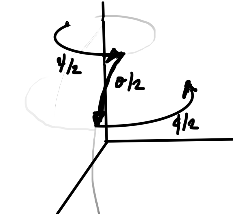
Here we used \( e^{\vcap \alpha} \gamma_0 = \gamma_0 e^{-\vcap \alpha} \), and \( \gpgradezero{A B} = \gpgradezero{B A} \). Geometrically, we have the curious fact that the direction vectors to points on the curve are perpendicular (with respect to our relativistic dot product) to the tangent vectors on the curve, as illustrated in fig. 1.

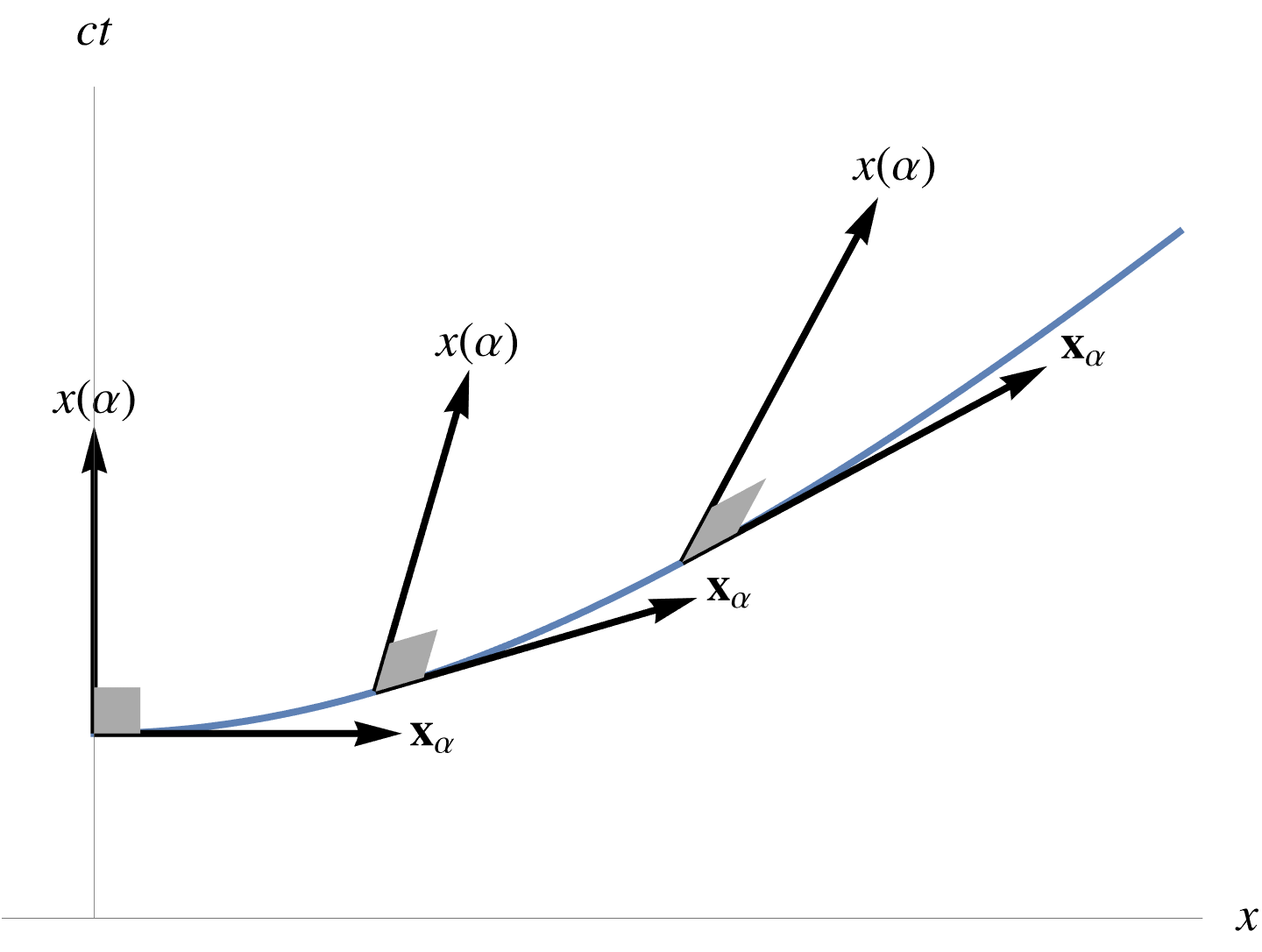
fig. 1. Tangent perpendicularity in mixed metric.

Perfect differentials.

Having seen a couple examples of multivector line integrals, let’s now move on to figure out the structure of a line integral that has a “perfect” differential integrand. We can take a hint from the \(\mathbb{R}^3\) vector result that we already know, namely
\begin{equation}\label{eqn:fundamentalTheoremOfGC:120}
\int_A^B d\Bl \cdot \spacegrad f = f(B) – f(A).
\end{equation}
It seems reasonable to guess that the relativistic generalization of this is
\begin{equation}\label{eqn:fundamentalTheoremOfGC:140}
\int_A^B dx \cdot \grad f = f(B) – f(A).
\end{equation}
Let’s check that, by expanding in coordinates
\begin{equation}\label{eqn:fundamentalTheoremOfGC:160}
\begin{aligned}
\int_A^B dx \cdot \grad f
&=
\int_A^B d\tau \frac{dx^\mu}{d\tau} \partial_\mu f \\
&=
\int_A^B d\tau \frac{dx^\mu}{d\tau} \PD{x^\mu}{f} \\
&=
\int_A^B d\tau \frac{df}{d\tau} \\
&=
f(B) – f(A).
\end{aligned}
\end{equation}
If we drop the dot product, will we have such a nice result? Let’s see:
\begin{equation}\label{eqn:fundamentalTheoremOfGC:180}
\begin{aligned}
\int_A^B dx \grad f
&=
\int_A^B d\tau \frac{dx^\mu}{d\tau} \gamma_\mu \gamma^\nu \partial_\nu f \\
&=
\int_A^B d\tau \frac{dx^\mu}{d\tau} \PD{x^\mu}{f}
+
\int_A^B
d\tau
\sum_{\mu \ne \nu} \gamma_\mu \gamma^\nu
\frac{dx^\mu}{d\tau} \PD{x^\nu}{f}.
\end{aligned}
\end{equation}
This scalar component of this integrand is a perfect differential, but the bivector part of the integrand is a complete mess, that we have no hope of generally integrating. It happens that if we consider one of the simplest parameterization examples, we can get a strong hint of how to generalize the differential operator to one that ends up providing a perfect differential. In particular, let’s integrate over a linear constant path, such as \( x(\tau) = \tau \gamma_0 \). For this path, we have
\begin{equation}\label{eqn:fundamentalTheoremOfGC:200a}
\begin{aligned}
\int_A^B dx \grad f
&=
\int_A^B \gamma_0 d\tau \lr{
\gamma^0 \partial_0 +
\gamma^1 \partial_1 +
\gamma^2 \partial_2 +
\gamma^3 \partial_3 } f \\
&=
\int_A^B d\tau \lr{
\PD{\tau}{f} +
\gamma_0 \gamma^1 \PD{x^1}{f} +
\gamma_0 \gamma^2 \PD{x^2}{f} +
\gamma_0 \gamma^3 \PD{x^3}{f}
}.
\end{aligned}
\end{equation}
Just because the path does not have any \( x^1, x^2, x^3 \) component dependencies does not mean that these last three partials are neccessarily zero. For example \( f = f(x(\tau)) = \lr{ x^0 }^2 \gamma_0 + x^1 \gamma_1 \) will have a non-zero contribution from the \( \partial_1 \) operator. In that particular case, we can easily integrate \( f \), but we have to know the specifics of the function to do the integral. However, if we had a differential operator that did not include any component off the integration path, we would ahve a perfect differential. That is, if we were to replace the gradient with the projection of the gradient onto the tangent space, we would have a perfect differential. We see that the function of the dot product in \ref{eqn:fundamentalTheoremOfGC:140} has the same effect, as it rejects any component of the gradient that does not lie on the tangent space.

Definition 1.2: Vector derivative.

Given a spacetime manifold parameterized by \( x = x(u^0, \cdots u^{N-1}) \), with tangent vectors \( \Bx_\mu = \PDi{u^\mu}{x} \), and reciprocal vectors \( \Bx^\mu \in \textrm{Span}\setlr{\Bx_\nu} \), such that \( \Bx^\mu \cdot \Bx_\nu = {\delta^\mu}_\nu \), the vector derivative is defined as
\begin{equation}\label{eqn:fundamentalTheoremOfGC:240a}
\partial = \sum_{\mu = 0}^{N-1} \Bx^\mu \PD{u^\mu}{}.
\end{equation}
Observe that if this is a full parameterization of the space (\(N = 4\)), then the vector derivative is identical to the gradient. The vector derivative is the projection of the gradient onto the tangent space at the point of evaluation.Furthermore, we designate \( \lrpartial \) as the vector derivative allowed to act bidirectionally, as follows
\begin{equation}\label{eqn:fundamentalTheoremOfGC:260a}
R \lrpartial S
=
R \Bx^\mu \PD{u^\mu}{S}
+
\PD{u^\mu}{R} \Bx^\mu S,
\end{equation}
where \( R, S \) are multivectors, and summation convention is implied. In this bidirectional action,
the vector factors of the vector derivative must stay in place (as they do not neccessarily commute with \( R,S\)), but the derivative operators apply in a chain rule like fashion to both functions.

Noting that \( \Bx_u \cdot \grad = \Bx_u \cdot \partial \), we may rewrite the scalar line integral identity \ref{eqn:fundamentalTheoremOfGC:140} as
\begin{equation}\label{eqn:fundamentalTheoremOfGC:220}
\int_A^B dx \cdot \partial f = f(B) – f(A).
\end{equation}
However, as our example hinted at, the fundamental theorem for line integrals has a multivector generalization that does not rely on a dot product to do the tangent space filtering, and is more powerful. That generalization has the following form.

Theorem 1.1: Fundamental theorem for line integrals.

Given multivector functions \( F, G \), and a single parameter curve \( x(u) \) with line element \( d^1 \Bx = \Bx_u du \), then
\begin{equation}\label{eqn:fundamentalTheoremOfGC:280a}
\int_A^B F d^1\Bx \lrpartial G = F(B) G(B) – F(A) G(A).
\end{equation}

Start proof:

Writing out the integrand explicitly, we find
\begin{equation}\label{eqn:fundamentalTheoremOfGC:340}
\int_A^B F d^1\Bx \lrpartial G
=
\int_A^B \lr{
\PD{\alpha}{F} d\alpha\, \Bx_\alpha \Bx^\alpha G
+
F d\alpha\, \Bx_\alpha \Bx^\alpha \PD{\alpha}{G }
}
\end{equation}
However for a single parameter curve, we have \( \Bx^\alpha = 1/\Bx_\alpha \), so we are left with
\begin{equation}\label{eqn:fundamentalTheoremOfGC:360}
\begin{aligned}
\int_A^B F d^1\Bx \lrpartial G
&=
\int_A^B d\alpha\, \PD{\alpha}{(F G)} \\
&=
\evalbar{F G}{B}

\evalbar{F G}{A}.
\end{aligned}
\end{equation}

End proof.

More to come.

In the next installment we will explore surface integrals in spacetime, and the generalization of the fundamental theorem to multivector space time integrals.

References

[1] Peeter Joot. Geometric Algebra for Electrical Engineers. Kindle Direct Publishing, 2019.

[2] A. Macdonald. Vector and Geometric Calculus. CreateSpace Independent Publishing Platform, 2012.

PHY2403H Quantum Field Theory. Lecture 19: Pauli matrices, Weyl spinors, SL(2,c), Weyl action, Weyl equation, Dirac matrix, Dirac action, Dirac Lagrangian. Taught by Prof. Erich Poppitz

November 24, 2018 phy2403 , , , , , , ,

[Here are my notes for lecture 19 of the UofT course PHY2403H, Quantum Field Theory, taught by Prof. Erich Poppitz, fall 2018.] For this lecture my notes are pdf only, due to length. While the after-class length was 8 pages, it ended up expanded to 17 pages by the time I finished making sense of the material.

These also include a portion of the notes from Lecture 18 (not yet posted), as it made sense to group all the Pauli matrix related content.  This particular set of notes diverges from the format presented in class, as it made sense to me to group things in this particular lecture in a more structured definition, theorem, proof style.  I’ve added a number of additional details that I found helpful, as well as a couple of extra problems (some set as formal problems at the end, and others set as theorem or lemmas in with the rest.)

PHY2403H Quantum Field Theory. Lecture 10: Lorentz boosts, generator of spacetime translation, Lorentz invariant field representation. Taught by Prof. Erich Poppitz

October 16, 2018 phy2403 , , , , ,

[Click here for a PDF of this post with nicer formatting]

DISCLAIMER: Very rough notes from class, with some additional side notes.

These are notes for the UofT course PHY2403H, Quantum Field Theory I, taught by Prof. Erich Poppitz fall 2018.

Lorentz transform symmetries.

From last time, recall that an infinitesimal Lorentz transform has the form
\begin{equation}\label{eqn:qftLecture10:20}
x^\mu \rightarrow x^\mu + \omega^{\mu\nu} x_\nu,
\end{equation}
where
\begin{equation}\label{eqn:qftLecture10:40}
\omega^{\mu\nu} = -\omega^{\nu\mu}
\end{equation}

We showed last time that \( \omega^{ij} \) induces a rotation, and will show today that \( \omega^{0i} \) is a boost.

We introduced a three index current, factoring out explicit dependence on the incremental Lorentz transform tensor \( \omega^{\mu\nu} \) as follows
\begin{equation}\label{eqn:qftLecture10:80}
J^{\nu \mu\rho} = \inv{2} \lr{ x^\rho T^{\nu\mu} – x^\mu T^{\nu\rho} },
\end{equation}
and can easily show that this current has the desired zero four-divergence property
\begin{equation}\label{eqn:qftLecture10:100}
\begin{aligned}
\partial_\nu J^{\nu \mu\rho}
&= \inv{2} \lr{
(\partial_\nu x^\rho) T^{\nu\mu}
+
x^\rho {\partial_\nu T^{\nu\mu} }
– (\partial_\nu x^\mu) T^{\nu\rho}
– x^\mu {\partial_\nu T^{\nu\rho} }
} \\
&= \inv{2} \lr{
(\partial_\nu x^\rho) T^{\nu\mu}
– (\partial_\nu x^\mu) T^{\nu\rho}
} \\
&= \inv{2} \lr{
T^{\rho\mu}
+
– T^{\mu\rho}
} \\
&= 0,
\end{aligned}
\end{equation}
since the energy-momentum tensor is symmetric.

Defining charge in the usual fashion \( Q = \int d^3 x j^0 \), so we can define a charge for each pair of indexes \( \mu\nu \), and in particular
\begin{equation}\label{eqn:qftLecture10:120}
Q^{0k} = \int d^3 x J^{0 0 k} = \inv{2} \int d^3 x \lr{ x^k T^{00} – x^0 T^{0k} }
\end{equation}
\begin{equation}\label{eqn:qftLecture10:540}
\begin{aligned}
\dot{Q}^{0k}
&= \int d^3 x \dot{J}^{0 0k} \\
&= \inv{2} \int d^3 x \lr{ x^k \dot{T}^{00} – x^0 \dot{T}^{0k} }
\end{aligned}
\end{equation}

However, since \( 0 = \partial_\mu T^{\mu \nu} = \dot{T}^{0 \nu} + \partial_j T^{j \nu} \), or \( \dot{T}^{0 \nu} = -\partial_j T^{j \nu} \),
\begin{equation}\label{eqn:qftLecture10:560}
\begin{aligned}
\dot{Q}^{0k}
&= \inv{2} \int d^3 x \lr{ x^k (-\partial_j T^{j0}) – T^{0k} – x^0 (-\partial_j T^{jk}) } \\
&= \inv{2} \int d^3 x \lr{
\partial_j (-x^k T^{j0}) + (\partial_j x^k) T^{j0}
– T^{0k} + x^0 \partial_j T^{jk}
} \\
&= \inv{2} \int d^3 x \lr{
\partial_j (-x^k T^{j0}) + {T^{k0}}
– {T^{0k}} + x^0 \partial_j T^{jk}
} \\
&= \inv{2} \int d^3 x \lr{
\partial_j (-x^k T^{j0})
+ x^0 \partial_j T^{jk}
} \\
&= \inv{2} \int d^3 x
\partial_j \lr{
-x^k T^{j0}
+ x^0 T^{jk}
},
\end{aligned}
\end{equation}
which leaves just surface terms, so \( \dot{Q}^{0k} = 0 \).

Quantizing:

From our previous identification
\begin{equation}\label{eqn:qftLecture9:560}

{T^\nu}_\mu =
-\partial^\nu \phi \partial_\mu \phi + {\delta^{\nu}}_\mu \LL,
\end{equation}
we have
\begin{equation}\label{eqn:qftLecture10:580}
T^{\nu\mu} = \partial^\nu \phi \partial^\mu \phi – g^{\nu\mu} \LL,
\end{equation}
or
\begin{equation}\label{eqn:qftLecture10:600}
\begin{aligned}
T^{00}
&= \partial^0 \phi \partial^0 \phi – \inv{2} \lr{ \partial_0 \phi \partial^0 \phi + \partial_k \phi \partial^k \phi } \\
&= \inv{2} \partial^0 \phi \partial^0 \phi – \inv{2} (\spacegrad \phi)^2,
\end{aligned}
\end{equation}
and
\begin{equation}\label{eqn:qftLecture10:620}
T^{0k} = \partial^0 \phi \partial^k \phi,
\end{equation}
so we may quantize these energy momentum tensor components as
\begin{equation}\label{eqn:qftLecture10:640}
\begin{aligned}
\hatT^{00} &= \inv{2} \hat{\pi}^2 + \inv{2} (\spacegrad \phihat)^2 \\
\hatT^{0k} &= \inv{2} \hat{\pi} \partial^k \phihat.
\end{aligned}
\end{equation}

We can now start computing the commutators associated with the charge operator. The first of those commutators is
\begin{equation}\label{eqn:qftLecture10:140}
\antisymmetric{\hatT^{00}(\Bx)}{\phihat(\By)}
=
\inv{2}
\antisymmetric{\hat{\pi}^2(\Bx)}{\phihat(\By)},
\end{equation}
which can be evaluated using the field commutator analogue of \( \antisymmetric{F(p)}{q} = i F’ \) which is
\begin{equation}\label{eqn:qftLecture10:660}
\antisymmetric{F(\hat{\pi}(\Bx))}{\phihat(\By)} = -i \frac{dF}{d \hat{\pi}} \delta(\Bx – \By),
\end{equation}
to give
\begin{equation}\label{eqn:qftLecture10:680}
\antisymmetric{\hatT^{00}(\Bx)}{\phihat(\By)}
= -i \delta^3(\Bx – \By) \hat{\pi}(\Bx)
\end{equation}

The other required commutator is
\begin{equation}\label{eqn:qftLecture10:160}
\begin{aligned}
\antisymmetric{\hatT^{0i}(\Bx)}{\phihat(\By)}
&=
\antisymmetric{\hat{\pi}(\Bx)\partial^i \phihat(\Bx)}{\phihat(\By)} \\
&=
\partial^i \phihat(\Bx)
\antisymmetric{\hat{\pi}(\Bx)
}{\phihat(\By)} \\
&= -i \delta^3(\Bx – \By) \partial^i \phihat(\Bx),
\end{aligned}
\end{equation}

The charge commutator with the field can now be computed
\begin{equation}\label{eqn:qftLecture10:180}
\begin{aligned}
i \epsilon \antisymmetric{\hatQ^{0k}}{\phihat(\By)}
&=
i
\frac{\epsilon}{2} \int d^3 x
\lr{
x^k
\antisymmetric{\hatT^{00}}{\phihat(\By)}

x^0
\antisymmetric{\hatT^{0k}}{\phihat(\By)}
} \\
&=
\frac{\epsilon}{2} \lr{ y^k \hat{\pi}(\By) – y^0 \partial^k \phihat(\By) } \\
&=
\frac{\epsilon}{2} \lr{ y^k \dot{\phihat}(\By) – y^0 \partial^k \phihat(\By) },
\end{aligned}
\end{equation}
so to first order in \( \epsilon \)
\begin{equation}\label{eqn:qftLecture10:200}
e^{i \epsilon \hatQ^{0k} } \phihat(\By)
e^{-i \epsilon \hatQ^{0k} }
=
\phihat(\By)
+ \frac{\epsilon}{2} y^k \dot{\phihat}(\By)
+ \frac{\epsilon}{2} y^0 \partial_k \phihat(\By)
\end{equation}

For example, with \( k = 1 \)
\begin{equation}\label{eqn:qftLecture10:700}
\begin{aligned}
e^{i \epsilon \hatQ^{0k} } \phihat(\By)
e^{-i \epsilon \hatQ^{0k} }
&=
\phihat(\By)
+ \frac{\epsilon}{2} \lr{
y^1 \dot{\phihat}(\By)
+
y^0 \PD{y^1}{\phihat}(\By)
} \\
&=
\phihat(y^0 + \frac{\epsilon}{2} y^1,
y^1 + \frac{\epsilon}{2} y^2, y^3).
\end{aligned}
\end{equation}

This is a boost. If we compare explicitly to an infinitesimal Lorentz transformation of the coordinates
\begin{equation}\label{eqn:qftLecture10:220}
\begin{aligned}
x^0 \rightarrow x^0 + \omega^{01} x_1 &= x^0 – \omega^{01} x^1 \\
x^1 \rightarrow x^1 + \omega^{10} x_0 &= x^1 – \omega^{01} x_0 = x^1 – \omega^{01} x^0
\end{aligned}
\end{equation}
we can make the identification
\begin{equation}\label{eqn:qftLecture10:240}
\frac{\epsilon}{2} = – \omega^{01}.
\end{equation}

We now have the explicit form of the generator of a spacetime translation

\begin{equation}\label{eqn:qftLecture10:260}
\boxed{
\hatU(\Lambda) = \exp\lr{-i \omega^{0k} \int d^3 x \lr{ \hatT^{00} x^k – \hatT^{0k} x^0 }}
}
\end{equation}

An explicit boost along the x-axis has the form
\begin{equation}\label{eqn:qftLecture10:300}
\hatU(\Lambda) \phihat(t, \Bx)
\hatU^\dagger(\Lambda)
=
\phihat\lr{ \frac{t – vx}{\sqrt{1 – v^2}}, \frac{x – vt}{\sqrt{1 – v^2}}, y, z },
\end{equation}
and more generally
\begin{equation}\label{eqn:qftLecture10:320}
\hatU(\Lambda) \phihat(x) \hatU^\dagger(\Lambda) =
\phihat(\Lambda x)
\end{equation}
where \( x \) is a four vector, \( (\Lambda x)^\mu = {{\Lambda}^\mu}_\nu x^\nu \), and \(
{{\Lambda}^\mu}_\nu
\approx
{{\delta}^\mu}_\nu
+
{{\omega}^\mu}_\nu \).

Transformation of momentum states

In the momentum space representation

\begin{equation}\label{eqn:qftLecture10:340}
\begin{aligned}
\phihat(x)
&=
\int \frac{d^3 p}{(2 \pi)^3 \sqrt{2 \omega_\Bp}} \lr{
e^{i (\omega_\Bp t – \Bp \cdot \Bx)} \hat{a}_\Bp
+
e^{-i (\omega_\Bp t – \Bp \cdot \Bx)} \hat{a}^\dagger_\Bp
} \\
&=
\int \frac{d^3 p}{(2 \pi)^3 \sqrt{2 \omega_\Bp}} \evalbar{
\lr{
e^{i p^\mu x^\mu } \hat{a}_\Bp
+
e^{-i p^\mu x^\mu } \hat{a}^\dagger_\Bp
}
}{p_0 = \omega_\Bp}
\end{aligned}
\end{equation}
\begin{equation}\label{eqn:qftLecture10:720}
\begin{aligned}
\hatU(\Lambda) \phihat(x) \hatU^\dagger(\Lambda)
&=
\phihat(\Lambda x) \\
&=
\int \frac{d^3 p}{(2 \pi)^3 \sqrt{2 \omega_\Bp}} \evalbar{
\lr{
e^{i p^\mu {{\Lambda}^\mu}_\nu x^\nu }
\hat{a}_\Bp
+
e^{-i p^\mu {{\Lambda}^\mu}_\nu x^\nu } \hat{a}^\dagger_\Bp
}
}{p_0 = \omega_\Bp}
\end{aligned}
\end{equation}
This can be put into an explicitly Lorentz invariant form
\begin{equation}\label{eqn:qftLecture10:n}
\begin{aligned}
\phihat(\Lambda x)
&=
\int \frac{dp^0 d^3 p}{(2\pi)^3} \delta(p_0^2 – \Bp^2 – m^2) \Theta(p^0) \sqrt{2 \omega_\Bp}
e^{i p^\mu {{\Lambda}^\mu}_\nu x^\nu }
\hat{a}_\Bp + \text{h.c.} \\
&=
\int \frac{dp^0 d^3 p}{(2\pi)^3}
\lr{
\frac{\delta(p_0 – \omega_\Bp)}{2 \omega_\Bp}
+
\frac{\delta(p_0 + \omega_\Bp)}{2 \omega_\Bp}
}
\Theta(p^0) \sqrt{2 \omega_\Bp} \hat{a}_\Bp + \text{h.c.},
\end{aligned}
\end{equation}
which recovers \ref{eqn:qftLecture10:720} by making use of the delta function identity \( \delta(f(x)) = \sum_{f(x_\conj) = 0} \frac{\delta(x – x_\conj)}{f'(x_\conj)} \), since the \( \Theta(p^0) \) kills the second delta function.

We now have a more explicit Lorentz invariant structure
\begin{equation}\label{eqn:qftLecture10:380}
\phihat(\Lambda x)
=
\int \frac{dp^0 d^3 p}{(2\pi)^3} \delta(p_0^2 – \Bp^2 – m^2) \Theta(p^0) \sqrt{2 \omega_\Bp}
e^{i p^\mu {{\Lambda}^\mu}_\nu x^\nu }
\hat{a}_\Bp + \text{h.c.}
\end{equation}

Recall that a boost moves a spacetime point along a parabola, such as that of fig. 1, whereas a rotation moves along a constant “circular” trajectory of a hyper-paraboloid. In general, a Lorentz transformation may move a spacetime point along any path on a hyper-paraboloid such as the one depicted (in two spatial dimensions) in fig. 2. This paraboloid depict the surfaces of constant energy-momentum \( p^0 = \sqrt{ \Bp^2 + m^2 } \). Because a Lorentz transformation only shift points along that energy-momentum surface, but cannot change the sign of the energy coordinate \( p^0 \), this means that \( \Theta(p^0) \) is also a Lorentz invariant.

fig. 1. One dimensional spacetime surface for constant (p^0)^2 – p^2 = m^2.


fig. 2. Surface of constant squared four-momentum.


Let’s change variables
\begin{equation}\label{eqn:qftLecture10:400}
p^\lambda = {{\Lambda}^\lambda}_\rho {p’}^{\rho}
\end{equation}
so that
\begin{equation}\label{eqn:qftLecture10:420}
\begin{aligned}
p_\mu
{{\Lambda}^\mu}_\nu x^\nu
&=
{{\Lambda}^\lambda}_\rho {p’}^\rho g_{\lambda\nu} {{\Lambda}^\nu}_\sigma x^{\sigma} \\
&=
{p’}^\rho
\lr{ {{\Lambda}^\lambda}_\rho
g_{\lambda\nu} {{\Lambda}^\nu}_\sigma } x^{\sigma} \\
&=
{p’}^\rho g_{\rho\sigma} x^\sigma
\end{aligned}
\end{equation}
which gives
\begin{equation}\label{eqn:qftLecture10:440}
\begin{aligned}
\phihat(\Lambda x)
&=
\int \frac{d{p’}^0 d^3 p’}{(2\pi)^3} \delta({p’}_0^2 – {\Bp’}^2 – m^2) \Theta(p^0) \sqrt{2 \omega_{\Lambda \Bp’}} e^{i p’ \cdot x} \hat{a}_{\Lambda \Bp’} + \text{h.c.} \\
&=
\int \frac{dp^0 d^3 p}{(2\pi)^3} \delta({p}_0^2 – {\Bp}^2 – m^2) \Theta(p^0) \sqrt{2 \omega_{\Lambda \Bp}} e^{i p \cdot x} \hat{a}_{\Lambda \Bp} + \text{h.c.}
\end{aligned}
\end{equation}
Since
\begin{equation}\label{eqn:qftLecture10:460}
\phihat(x)
=
\int \frac{dp^0 d^3 p}{(2\pi)^3} \delta({p}_0^2 – {\Bp}^2 – m^2) \Theta(p^0) \sqrt{2 \omega_{\Bp}} e^{i p \cdot x} \hat{a}_{\Bp} + \text{h.c.}
\end{equation}
we can now conclude that the creation and annihilation operators transform as

\begin{equation}\label{eqn:qftLecture10:480}
\boxed{
\sqrt{2 \omega_{\Lambda \Bp}} \hat{a}_{\Lambda \Bp}
=
\hatU(\Lambda)
\sqrt{2 \omega_{ \Bp}} \hat{a}_{ \Bp}
\hatU^\dagger(\Lambda)
}
\end{equation}

In particular
\begin{equation}\label{eqn:qftLecture10:500}
\sqrt{2 \omega_{ \Bp}} \hat{a}^\dagger_{ \Bp} \ket{0} = \ket{\Bp}
\end{equation}
and noting that \( \hatU(\Lambda) \ket{0} = \ket{0} \) (i.e. the ground state is Lorentz invariant), we have
\begin{equation}\label{eqn:qftLecture10:520}
\begin{aligned}
\sqrt{2 \omega_{\Lambda \Bp}} \hat{a}^\dagger_{\Lambda \Bp} \ket{0}
&=
\hatU(\Lambda) \sqrt{ 2\omega_\Bp} \hat{a}^\dagger_\Bp \hatU^\dagger(\Lambda) \hatU(\Lambda) \ket{0} \\
&=
\hatU(\Lambda) \sqrt{ 2\omega_\Bp} \hat{a}^\dagger_\Bp \ket{0} \\
&=
\hatU(\Lambda) \ket{\Bp}.
\end{aligned}
\end{equation}

PHY2403H Quantum Field Theory. Lecture 9: Unbroken and spontaneously broken symmetries, Higgs Lagrangian, scale invariance, Lorentz invariance, angular momentum quantization. Taught by Prof. Erich Poppitz

October 11, 2018 phy2403 , , , , , , , , , , , , , , ,

[Click here for a PDF of this post with nicer formatting (and a Mathematica listing that I didn’t include in this blog post’s latex export)]

DISCLAIMER: Very rough notes from class, with some additional side notes.

These are notes for the UofT course PHY2403H, Quantum Field Theory I, taught by Prof. Erich Poppitz fall 2018.

Last time

We followed a sequence of operations

  1. Noether’s theorem
  2. \( \rightarrow \) conserved currents
  3. \( \rightarrow \) charges (classical)
  4. \( \rightarrow \) “correspondence principle”
  5. \( \rightarrow \hatQ \)
  • Hermitian operators
  • “generators of symmetry”
    \begin{equation}\label{eqn:qftLecture9:20}
    \hatU(\alpha) = e^{i \alpha \hatQ}
    \end{equation}
    We found
    \begin{equation}\label{eqn:qftLecture9:40}
    \hatU(\alpha) \phihat \hatU^\dagger(\alpha) = \phihat + i \alpha \antisymmetric{\hatQ}{\phihat} + \cdots
    \end{equation}

Example: internal symmetries:

(non-spacetime), such as \( O(N)\) or \( U(1) \).

In QFT internal symmetries can have different “\underline{modes of realization}”.

    [I]

  1. “Wigner mode”. These are also called “unbroken symmetries”.
    \begin{equation}\label{eqn:qftLecture9:60}
    \hatQ \ket{0} = 0
    \end{equation}
    i.e. \( \hatU(\alpha) \ket{0} = 0 \).
    Ground state invariant. Formally \( :\hatQ: \) annihilates \( \ket{0} \).
    \( \antisymmetric{\hatQ}{\hatH} = 0 \) implies that all eigenstates are eigenstates of \( \hatQ \) in \( U(1) \). Example from HW 1
    \begin{equation}\label{eqn:qftLecture9:80}
    \hatQ = \text{“charge” under \( U(1) \)}.
    \end{equation}
    All states have definite charge, just live in QU.
  2. “Nambu-Goldstone mode” (Landau-ginsburg). This is also called a “spontaneously broken symmetry”\footnote{
    First encounter example (HWII, \( SU(2) \times SU(2) \rightarrow SU(2) \)). Here a \( U(1) \) spontaneous broken symmetry.}.
    \( H \) or \( L \) is invariant under symmetry, but ground state is not.

fig. 1. Mexican hat potential.

fig. 2. Degenerate Mexican hat potential ( v = 0)

Example:
\begin{equation}\label{eqn:qftLecture9:100}
\LL = \partial_\mu \phi^\conj \partial^\mu \phi – V(\Abs{\phi}),
\end{equation}
where
\begin{equation}\label{eqn:qftLecture9:120}
V(\Abs{\phi}) = m^2 \phi^\conj \phi + \frac{\lambda}{4} \lr{ \phi^\conj \phi }^2.
\end{equation}
When \( m^2 > 0 \) we have a Wigner mode, but when \( m^2 < 0 \) we have an issue: \( \phi = 0 \) is not a minimum of potential.
When \( m^2 < 0 \) we write
\begin{equation}\label{eqn:qftLecture9:140}
\begin{aligned}
V(\phi)
&= – m^2 \phi^\conj \phi + \frac{\lambda}{4} \lr{ \phi^\conj \phi}^2 \\
&= \frac{\lambda}{4} \lr{
\lr{ \phi^\conj \phi}^2 – \frac{4}{\lambda} m^2 } \\
&= \frac{\lambda}{4} \lr{
\phi^\conj \phi – \frac{2}{\lambda} m^2 }^2 – \frac{4 m^4}{\lambda^2},
\end{aligned}
\end{equation}
or simply
\begin{equation}\label{eqn:qftLecture9:780}
V(\phi)
=
\frac{\lambda}{4} \lr{ \phi^\conj \phi – v^2 }^2 + \text{const}.
\end{equation}
The potential (called the Mexican hat potential) is illustrated in fig. 1 for non-zero \( v \), and in
fig. 2 for \( v = 0 \).
We choose to expand around some point on the minimum ring (it doesn’t matter which one).
When there is no potential, we call the field massless (i.e. if we are in the minimum ring).
We expand as
\begin{equation}\label{eqn:qftLecture9:160}
\phi(x) = v \lr{ 1 + \frac{\rho(x)}{v} } e^{i \alpha(x)/v },
\end{equation}
so
\begin{equation}\label{eqn:qftLecture9:180}
\begin{aligned}
\frac{\lambda}{4}
\lr{\phi^\conj \phi – v^2}^2
&=
\lr{
v^2 \lr{ 1 + \frac{\rho(x)}{v} }^2
– v^2
}^2 \\
&=
\frac{\lambda}{4}
v^4 \lr{ \lr{ 1 + \frac{\rho(x)}{v} }^2 – 1 } \\
&=
\frac{\lambda}{4}
v^4
\lr{
\frac{2 \rho}{v} + \frac{\rho^2}{v^2}
}^2.
\end{aligned}
\end{equation}

\begin{equation}\label{eqn:qftLecture9:200}
\partial_\mu \phi =
\lr{
v \lr{ 1 + \frac{\rho(x)}{v} } \frac{i}{v} \partial_\mu \alpha
+ \partial_\mu \rho
} e^{i \alpha}
\end{equation}

so
\begin{equation}\label{eqn:qftLecture9:220}
\begin{aligned}
\LL
&= \Abs{\partial \phi^\conj}^2 – \frac{\lambda}{4} \lr{ \Abs{\phi^\conj}^2 – v^2 }^2 \\
&=
\partial_\mu \rho \partial^\mu \rho + \partial_\mu \alpha \partial^\mu \alpha \lr{ 1 + \frac{\rho}{v} }

\frac{\lambda v^4}{4} \frac{ 4\rho^2}{v^2} + O(\rho^3) \\
&=
\partial_\mu \rho \partial^\mu \rho
– \lambda v^2\rho^2
+
\partial_\mu \alpha \partial^\mu \alpha \lr{ 1 + \frac{\rho}{v} }.
\end{aligned}
\end{equation}
We have two fields, \( \rho \) : a massive scalar field, the “Higgs”, and a massless field \( \alpha \) (the Goldstone Boson).

\( U(1) \) symmetry acts on \( \phi(x) \rightarrow e^{i \omega } \phi(x) \) i.t.o \( \alpha(x) \rightarrow \alpha(x) + v \omega \).
\( U(1) \) global symmetry (broken) acts on the Goldstone field \( \alpha(x) \) by a constant shift. (\(U(1)\) is still a symmetry of the Lagrangian.)

The current of the \( U(1) \) symmetry is:
\begin{equation}\label{eqn:qftLecture9:240}
j_\mu = \partial_\mu \alpha \lr{ 1 + \text{higher dimensional \( \rho \) terms} }.
\end{equation}

When we quantize
\begin{equation}\label{eqn:qftLecture9:260}
\alpha(x) =
\int \frac{d^3p}{(2\pi)^3 \sqrt{ 2 \omega_p }} e^{i \omega_p t – i \Bp \cdot \Bx} \hat{a}_\Bp^\dagger +
\int \frac{d^3p}{(2\pi)^3 \sqrt{ 2 \omega_p }} e^{-i \omega_p t + i \Bp \cdot \Bx} \hat{a}_\Bp
\end{equation}
\begin{equation}\label{eqn:qftLecture9:280}
j^\mu(x) = \partial^\mu \alpha(x) =
\int \frac{d^3p}{(2\pi)^3 \sqrt{ 2 \omega_p }} \lr{ i \omega_\Bp – i \Bp } e^{i \omega_p t – i \Bp \cdot \Bx} \hat{a}_\Bp^\dagger +
\int \frac{d^3p}{(2\pi)^3 \sqrt{ 2 \omega_p }} \lr{ -i \omega_\Bp + i \Bp } e^{-i \omega_p t + i \Bp \cdot \Bx} \hat{a}_\Bp.
\end{equation}

\begin{equation}\label{eqn:qftLecture9:300}
j^\mu(x) \ket{0} \ne 0,
\end{equation}
instead it creates a single particle state.

Examples of symmetries

In particle physics, examples of Wigner vs Nambu-Goldstone, ignoring gravity the only exact internal symmetry in the standard module is
\( (B\# – L\#) \), believed to be a \( U(1) \) symmetry in Wigner mode.

Here \(B\#\) is the Baryon number, and \( L\# \) is the Lepton number. Examples:

  • \( B(p) = 1 \), proton.
  • \( B(q) = 1/3 \), quark
  • \( B(e) = 1 \), electron
  • \( B(n) = 1 \), neutron.
  • \( L(p) = 1 \), proton.
  • \( L(q) = 0 \), quark.
  • \( L(e) = 0 \), electron.

The major use of global internal symmetries in the standard model is as “approximate” ones. They become symmetries when one neglects some effect( “terms in \( \LL \)”).
There are other approximate symmetries (use of group theory to find the Balmer series).

Example from HW2:

QCD in limit
\begin{equation}\label{eqn:qftLecture9:320}
m_u = m_d = 0.
\end{equation}
\( m_u m_d \ll m_p \) (the products of the up-quark mass and the down-quark mass are much less than a composite one (name?)).
\( SU(2)_L \times SU(2)_R \rightarrow SU(2)_V \)

EWSB (Electro-Weak-Symmetry-Breaking) sector

When the couplings \( g_2, g_1 = 0 \). (\( g_2 \in SU(2), g_1 \in U(1) \)).

Scale invariance

\begin{equation}\label{eqn:qftLecture9:340}
\begin{aligned}
x &\rightarrow e^{\lambda} x \\
\phi &\rightarrow e^{-\lambda} \phi \\
A_\mu &\rightarrow e^{-\lambda} A_\mu
\end{aligned}
\end{equation}
Any unitary theory which is scale invariant is also \underline{conformal} invariant. Conformal invariance means that angles are preserved.
The point here is that there is more than scale invariance.

We have classical internal global continuous symmetries.
These can be either

  1. “unbroken” (Wigner mode)
    \begin{equation}\label{eqn:qftLecture9:360}
    \hatQ\ket{0} = 0.
    \end{equation}
  2. “spontaneously broken”
    \begin{equation}\label{eqn:qftLecture9:380}
    j^\mu(x) \ket{0} \ne 0
    \end{equation}
    (creates Goldstone modes).
  3. “anomalous”. Classical symmetries are not a symmetry of QFT.
    Examples:

    • Scale symmetry (to be studied in QFT II), although this is not truly internal.
    • In QCD again when \( \omega_\Bq = 0 \), a \( U(1\) symmetry (chiral symmetry) becomes exact, and cannot be preserved in QFT.
    • In the standard model (E.W sector), the Baryon number and Lepton numbers are not symmetries, but their difference \( B\# – L\# \) is a symmetry.

Lorentz invariance.

We’d like to study the action of Lorentz symmetries on quantum states. We are going to “go by the book”, finding symmetries, currents, quantize, find generators, and so forth.

Under a Lorentz transformation
\begin{equation}\label{eqn:qftLecture9:400}
x^\mu \rightarrow {x’}^\mu = {\Lambda^\mu}_\nu x^\nu,
\end{equation}
We are going to consider infinitesimal Lorentz transformations
\begin{equation}\label{eqn:qftLecture9:420}
{\Lambda^\mu}_\nu \approx
{\delta^\mu}_\nu + {\omega^\mu}_\nu
,
\end{equation}
where \( {\omega^\mu}_\nu \) is small.
A Lorentz transformation \( \Lambda \) must satisfy \( \Lambda^\T G \Lambda = G \), or
\begin{equation}\label{eqn:qftLecture9:800}
g_{\mu\nu} = {{\Lambda}^\alpha}_\mu g_{\alpha \beta} {{\Lambda}^\beta}_\nu,
\end{equation}
into which we insert the infinitesimal transformation representation
\begin{equation}\label{eqn:qftLecture9:820}
\begin{aligned}
0
&=
– g_{\mu\nu} +
\lr{ {\delta^\alpha}_\mu + {\omega^\alpha}_\mu }
g_{\alpha \beta}
\lr{ {\delta^\beta}_\nu + {\omega^\beta}_\nu } \\
&=
– g_{\mu\nu} +
\lr{
g_{\mu \beta}
+
\omega_{\beta\mu}
}
\lr{ {\delta^\beta}_\nu + {\omega^\beta}_\nu } \\
&=
– g_{\mu\nu} +
g_{\mu \nu}
+
\omega_{\nu\mu}
+
\omega_{\mu\nu}
+
\omega_{\beta\mu}
{\omega^\beta}_\nu.
\end{aligned}
\end{equation}
The quadratic term can be ignored, leaving just
\begin{equation}\label{eqn:qftLecture9:840}
0 =
\omega_{\nu\mu}
+
\omega_{\mu\nu},
\end{equation}
or
\begin{equation}\label{eqn:qftLecture9:860}
\omega_{\nu\mu} = – \omega_{\mu\nu}.
\end{equation}
Note that \( \omega \) is a completely antisymmetric tensor, and like \( F_{\mu\nu} \) this has only 6 elements.
This means that the
infinitesimal transformation of the coordinates is
\begin{equation}\label{eqn:qftLecture9:440}
x^\mu \rightarrow {x’}^\mu \approx x^\mu + \omega^{\mu\nu} x_\nu,
\end{equation}
the field transforms as
\begin{equation}\label{eqn:qftLecture9:460}
\phi(x) \rightarrow \phi'(x’) = \phi(x)
\end{equation}
or
\begin{equation}\label{eqn:qftLecture9:760}
\phi'(x^\mu + \omega^{\mu\nu} x_\nu) =
\phi'(x) + \omega^{\mu\nu} x_\nu \partial_\mu\phi(x) = \phi(x),
\end{equation}
so
\begin{equation}\label{eqn:qftLecture9:480}
\delta \phi = \phi'(x) – \phi(x) =
-\omega^{\mu\nu} x_\nu \partial_\mu \phi.
\end{equation}

Since \( \LL \) is a scalar
\begin{equation}\label{eqn:qftLecture9:500}
\begin{aligned}
\delta \LL
&=
-\omega^{\mu\nu} x_\nu \partial_\mu \LL \\
&=

\partial_\mu \lr{
\omega^{\mu\nu} x_\nu \LL
}
+
(\partial_\mu x_\nu) \omega^{\mu\nu} \LL \\
&=
\partial_\mu \lr{

\omega^{\mu\nu} x_\nu \LL
},
\end{aligned}
\end{equation}
since \( \partial_\nu x_\mu = g_{\nu\mu} \) is symmetric, and \( \omega \) is antisymmetric.
Our current is
\begin{equation}\label{eqn:qftLecture9:520}
J^\mu_\omega
=

\omega^{\mu\nu} x_\mu \LL
.
\end{equation}
Our Noether current is
\begin{equation}\label{eqn:qftLecture9:540}
\begin{aligned}
j^\nu_{\omega^{\mu\rho}}
&= \PD{\phi_{,\nu}}{\LL} \delta \phi – J^\mu_\omega \\
&=
\partial^\nu \phi\lr{ – \omega^{\mu\rho} x_\rho \partial_\mu \phi } + \omega^{\nu \rho} x_\rho \LL \\
&=
\omega^{\mu\rho}
\lr{
\partial^\nu \phi\lr{ – x_\rho \partial_\mu \phi } + {\delta^{\nu}}_\mu x_\rho \LL
} \\
&=
\omega^{\mu\rho} x_\rho
\lr{
-\partial^\nu \phi \partial_\mu \phi + {\delta^{\nu}}_\mu \LL
}
\end{aligned}
\end{equation}
We identify
\begin{equation}\label{eqn:qftLecture9:560}

{T^\nu}_\mu =
-\partial^\nu \phi \partial_\mu \phi + {\delta^{\nu}}_\mu \LL,
\end{equation}
so the current is
\begin{equation}\label{eqn:qftLecture9:580}
\begin{aligned}
j^\nu_{\omega_{\mu\rho}}
&=
-\omega^{\mu\rho} x_\rho
{T^\nu}_\mu \\
&=
-\omega_{\mu\rho} x^\rho
T^{\nu\mu}
.
\end{aligned}
\end{equation}
Define
\begin{equation}\label{eqn:qftLecture9:600}
j^{\nu\mu\rho} = \inv{2} \lr{ x^\rho T^{\nu\mu} – x^{\mu} T^{\nu\rho} },
\end{equation}
which retains the antisymmetry in \( \mu \rho \) yet still drops the parameter \( \omega^{\mu\rho} \).
To check that this makes sense, we can contract
\( j^{\nu\mu\rho} \) with \( \omega_{\rho\mu} \)
\begin{equation}\label{eqn:qftLecture9:880}
\begin{aligned}
j^{\nu\mu\rho} \omega_{\rho\mu}
&= -\inv{2} \lr{ x^\rho T^{\nu\mu} – x^{\mu} T^{\nu\rho} }
\omega_{\mu\rho} \\
&=
-\inv{2} x^\rho T^{\nu\mu}
\omega_{\mu\rho}
– \inv{2} x^{\mu} T^{\nu\rho}
\omega_{\rho\mu} \\
&=
-\inv{2} x^\rho T^{\nu\mu}
\omega_{\mu\rho}
– \inv{2} x^{\rho} T^{\nu\mu}
\omega_{\mu\rho} \\
&=
– x^{\rho} T^{\nu\mu}
\omega_{\mu\rho},
\end{aligned}
\end{equation}
which matches \ref{eqn:qftLecture9:580} as desired.

Example. Rotations \( \mu\rho = ij \)

\begin{equation}\label{eqn:qftLecture9:620}
\begin{aligned}
J^{0 i j} \epsilon_{ijk}
&=
\inv{2} \lr{ x^i T^{0j} – x^{j} T^{0i} } \epsilon_{ijk} \\
&=
x^i T^{0j} \epsilon_{ijk}.
\end{aligned}
\end{equation}
Observe that this has the structure of \( (\Bx \cross \Bp)_k \), where \( \Bp \) is the momentum density of the field.
Let
\begin{equation}\label{eqn:qftLecture9:640}
L_k \equiv Q_k = \int d^3 x J^{0ij} \epsilon_{ijk}.
\end{equation}
We can now quantize and build a generator
\begin{equation}\label{eqn:qftLecture9:660}
\begin{aligned}
\hatU(\Balpha)
&= e^{i \Balpha \cdot \hat{\BL}} \\
&= \exp\lr{i \alpha_k
\int d^3 x x^i \hat{T}^{0j} \epsilon_{ijk}
}
\end{aligned}
\end{equation}
From \ref{eqn:qftLecture9:560} we can quantize with \( T^{0j} = \partial^0 \phi \partial^j \phi \rightarrow \hat{\pi} \lr{\spacegrad \phihat}_j\), or
\begin{equation}\label{eqn:qftLecture9:900}
\begin{aligned}
\hatU(\Balpha)
&=
\exp\lr{i \alpha_k
\int d^3 x x^i \hat{\pi} (\spacegrad \phihat)_j \epsilon_{ijk}
} \\
&=
\exp\lr{i \Balpha \cdot
\int d^3 x \hat{\pi} \spacegrad \phihat \cross \Bx
}
\end{aligned}
\end{equation}
(up to a sign in the exponent which doesn’t matter)
\begin{equation}\label{eqn:qftLecture9:680}
\begin{aligned}
\phihat(\By) \rightarrow \hatU(\alpha) \phihat(\By) \hatU^\dagger(\alpha)
&\approx
\phihat(\By) +
i \Balpha \cdot
\antisymmetric{
\int d^3 x \hat{\pi}(\Bx) \spacegrad \phihat(\Bx) \cross \Bx
}
{
\phihat(\By)
} \\
&=
\phihat(\By) +
i \Balpha \cdot
\int d^3 x
(-i) \delta^3(\Bx – \By)
\spacegrad \phihat(\Bx) \cross \Bx \\
&=
\phihat(\By) +
\Balpha \cdot \lr{ \spacegrad \phihat(\By ) \cross \By}
\end{aligned}
\end{equation}
Explicitly, in coordinates, this is
\begin{equation}\label{eqn:qftLecture9:700}
\begin{aligned}
\phihat(\By)
&\rightarrow
\phihat(\By) +
\alpha^i
\lr{
\partial^j \phihat(\By) y^k \epsilon_{jki}
} \\
&=
\phihat(\By) –
\epsilon_{ikj} \alpha^i y^k \partial^j \phihat \\
&=
\phihat( y^j – \epsilon^{ikj} \alpha^i y^k ).
\end{aligned}
\end{equation}
This is a rotation. To illustrate, pick \( \Balpha = (0, 0, \alpha) \), so \( y^j \rightarrow y^j – \epsilon^{ikj} \alpha y^k \delta_{i3} = y^j – \epsilon^{3kj} \alpha y^k \), or
\begin{equation}\label{eqn:qftLecture9:n}
\begin{aligned}
y^1 &\rightarrow y^1 – \epsilon^{3k1} \alpha y^k = y^1 + \alpha y^2 \\
y^2 &\rightarrow y^2 – \epsilon^{3k2} \alpha y^k = y^2 – \alpha y^1 \\
y^3 &\rightarrow y^3 – \epsilon^{3k3} \alpha y^k = y^3,
\end{aligned}
\end{equation}
or in matrix form
\begin{equation}\label{eqn:qftLecture9:720}
\begin{bmatrix}
y^1 \\
y^2 \\
y^3 \\
\end{bmatrix}
\rightarrow
\begin{bmatrix}
1 & \alpha & 0 \\
-\alpha & 1 & 0 \\
0 & 0 & 1
\end{bmatrix}
\begin{bmatrix}
y^1 \\
y^2 \\
y^3 \\
\end{bmatrix}.
\end{equation}