math and physics play

ECE1254H Modeling of Multiphysics Systems. Lecture 19: Model order reduction (cont).. Taught by Prof. Piero Triverio

November 26, 2014 ece1254 , , ,

[Click here for a PDF of this post with nicer formatting]

Disclaimer

Peeter’s lecture notes from class. These may be incoherent and rough.

Model order reduction (cont).

An approximation of the following system is sought

\begin{equation}\label{eqn:multiphysicsL19:20}
\BG \Bx(t) + C \dot{\Bx}(t) = B \Bu(t)
\end{equation}
\begin{equation}\label{eqn:multiphysicsL19:40}
\By(t) = \BL^\T \Bx(t).
\end{equation}

The strategy is to attempt to find a \( N \times q \) projector \( \BV \) of the form

\begin{equation}\label{eqn:multiphysicsL19:60}
\BV =
\begin{bmatrix}
\Bv_1 & \Bv_2 & \cdots & \Bv_q
\end{bmatrix}
\end{equation}

so that the solution of the constrained q-variable state vector \( \Bx_q \) is sought after letting

\begin{equation}\label{eqn:multiphysicsL19:80}
\Bx(t) = \BV \Bx_q(t).
\end{equation}

Moment matching

\begin{equation}\label{eqn:multiphysicsL19:100}
\begin{aligned}
\BF(s)
&= \lr{ \BG + s \BC }^{-1} \BB \\
&= \BM_0 + \BM_1 s + \BM_2 s^2 + \cdots + \BM_{q-1} s^{q-1} + M_q s^q + \cdots
\end{aligned}
\end{equation}

The reduced model is created such that

\begin{equation}\label{eqn:multiphysicsProblemSet3b:120}
\BF_q(s)
=
\BM_0 + \BM_1 s + \BM_2 s^2 + \cdots + \BM_{q-1} s^{q-1} + \tilde{\BM}_q s^q.
\end{equation}

Form an \( N \times q \) projection matrix

\begin{equation}\label{eqn:multiphysicsL19:140}
\BV_q \equiv
\begin{bmatrix}
\BM_0 & \BM_1 & \cdots & \BM_{q-1}
\end{bmatrix}
\end{equation}

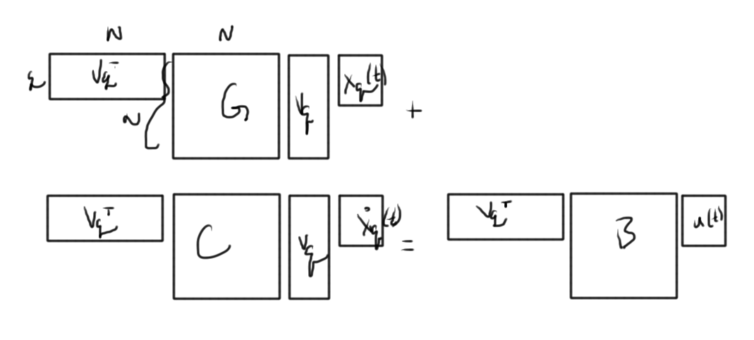
With the substitution of fig. 1, becomes

lecture19Fig1

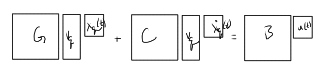
This is a system of \( N \) equations, in \( q \) unknowns. A set of moments from the frequency domain have been used to project the time domain system. This relies on the following unproved theorem (references to come)

Theorem

If \( \text{span}\{ \Bv_q \} = \text{span} \{ \BM_0, \BM_1, \cdots, \BM_{q-1} \} \), then the reduced model will match the first \( q \) moments.

Left multiplication by \( \BV_q^\T \) yields fig. 2.

lecture19Fig2

This is now a system of \( q \) equations in \( q \) unknowns.

With

\begin{equation}\label{eqn:multiphysicsL19:160}
\BG_q = \BV_q^\T \BG \BV_q
\end{equation}
\begin{equation}\label{eqn:multiphysicsL19:180}
\BC_q = \BV_q^\T \BC \BV_q
\end{equation}
\begin{equation}\label{eqn:multiphysicsL19:200}
\BB_q = \BV_q^\T \BB
\end{equation}
\begin{equation}\label{eqn:multiphysicsL19:220}
\BL_q^\T = \BL^\T \BV_q
\end{equation}

the system is reduced to

\begin{equation}\label{eqn:multiphysicsL19:240}
\BG_q \Bx_q(t) + \BC_q \dot{\Bx}_q(t) = \BB_q \Bu(t).
\end{equation}
\begin{equation}\label{eqn:multiphysicsL19:260}
\By(t) \approx \BL_q^\T \Bx_q(t)
\end{equation}

Moments calculation

Using
\begin{equation}\label{eqn:multiphysicsL19:300}
\lr{ \BG + s \BC }^{-1} \BB = \BM_0 + \BM_1 s + \BM_2 s^2 + \cdots
\end{equation}

thus
\begin{equation}\label{eqn:multiphysicsL19:320}
\begin{aligned}
\BB &=
\lr{ \BG + s \BC }
\BM_0 +
\lr{ \BG + s \BC }
\BM_1 s +
\lr{ \BG + s \BC }
\BM_2 s^2 + \cdots \\
&=
\BG \BM_0
+ s \lr{ C \BM_0 + \BG \BM_1 }
+ s^2 \lr{ C \BM_1 + \BG \BM_2 }
+ \cdots
\end{aligned}
\end{equation}

Since \( \BB \) is a zeroth order matrix, setting all the coefficients of \( s \) equal to zero provides a method to solve for the moments

\begin{equation}\label{eqn:multiphysicsL19:340}
\begin{aligned}
\BB &= \BG \BM_0 \\
-\BC \BM_0 &= \BG \BM_1 \\
-\BC \BM_1 &= \BG \BM_2 \\
\end{aligned}
\end{equation}

The moment \( \BM_0 \) can be found with LU of \( \BG \), plus the forward and backward substitutions. Proceeding recursively, using the already computed LU factorization, each subsequent moment calculation requires only one pair of forward and backward substitutions.

Numerically, each moment has the exact value

\begin{equation}\label{eqn:multiphysicsL19:360}
\BM_q = \lr{- \BG^{-1} \BC }^q \BM_0.
\end{equation}

As \( q \rightarrow \infty \), this goes to some limit, say \( \Bw \). The value \( \Bw \) is related to the largest eigenvalue of \( -\BG^{-1} \BC \). Incidentally, this can be used to find the largest eigenvalue of \( -\BG^{-1} \BC \).

The largest eigenvalue of this matrix will dominate these factors, and can cause some numerical trouble. For this reason it is desirable to avoid such explicit moment determination, instead using implicit methods.

The key is to utilize the theorem above, and look instead for an alternate basis \( \{ \Bv_q \} \) that also spans \( \{ \BM_0, \BM_1, \cdots, \BM_q \} \).

Space generate by the moments

Write

\begin{equation}\label{eqn:multiphysicsL19:380}
\BM_q = \BA^q \BR,
\end{equation}

where in this case

\begin{equation}\label{eqn:multiphysicsL19:400}
\begin{aligned}
\BA &= – \BG^{-1} \BC \\
\BR &= \BM_0 = -\BG \BB
\end{aligned}
\end{equation}

The span of interest is

\begin{equation}\label{eqn:multiphysicsL19:420}
\text{span} \{ \BR, \BA \BR, \BA^2 \BR, \cdots, \BA^{q-1} \BR \}.
\end{equation}

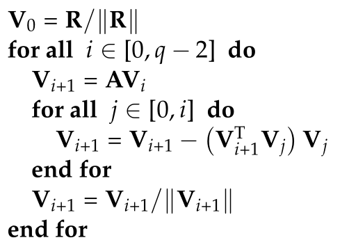
Such a sequence is called a Krylov subspace. One method to compute such a basis, the Arnoldi process, relies on Gram-Schmidt orthonormalization methods:

arnoldi

Some numerical examples and plots on the class slides.

Stability of discretized linear differential equations

November 17, 2014 ece1254 , , , ,

[Click here for a PDF of this post with nicer formatting]

In class today was a highlight of stability methods for linear multistep methods. To motivate the methods used, it is helpful to take a step back and review stability concepts for LDE systems.

By way of example, consider a second order LDE homogeneous system defined by

\begin{equation}\label{eqn:stabilityLDEandDiscreteTime:20}
\frac{d^2 x}{dt^2} + 3 \frac{dx}{dt} + 2 = 0.
\end{equation}

Such a system can be solved by assuming an exponential solution, say

\begin{equation}\label{eqn:stabilityLDEandDiscreteTime:40}
x(t) = e^{s t}.
\end{equation}

Substitution gives

\begin{equation}\label{eqn:stabilityLDEandDiscreteTime:60}
e^{st} \lr{ s^2 + 3 s + 2 } = 0,
\end{equation}

The polynomial part of this equation, the characteristic equation has roots \( s = -2, -1 \).

The general solution of \ref{eqn:stabilityLDEandDiscreteTime:20} is formed by a superposition of solutions for each value of \(s\)

\begin{equation}\label{eqn:stabilityLDEandDiscreteTime:80}
x(t) = a e^{-2 t} + b e^{-t}.
\end{equation}

Independent of any selection of the superposition constants \( a, b \), this function will not blow up as \( t \rightarrow \infty \).

This “stability” is due to the fact that both of the characteristic equation roots lie in the left hand Argand plane.

Now consider a discretized form of this LDE. This will have the form

\begin{equation}\label{eqn:stabilityLDEandDiscreteTime:100}
\begin{aligned}
0 &=
\inv{\lr{\Delta t}^2}
\lr{ x_{n+2} – 2 x_{n-1} + x_n } + \frac{3}{\Delta t} \lr{ x_{n+1} – x_n } + 2
x_n \\
&=
x_{n+2} \lr{
\inv{\lr{\Delta t}^2}
}
+
x_{n+1} \lr{
\frac{3}{\Delta t}
-\frac{2}{\lr{\Delta t}^2}
}
+
x_{n} \lr{
\frac{1}{\lr{\Delta t}^2}
-\frac{3}{\Delta t}
+ 2
},
\end{aligned}
\end{equation}

or

\begin{equation}\label{eqn:stabilityLDEandDiscreteTime:220}
0
=
x_{n+2}
+
x_{n+1} \lr{
3 \Delta t – 2
}
+
x_{n} \lr{
1 – 3 \Delta t + 2 \lr{ \Delta t}^2
}.
\end{equation}

Note that after discretization, each subsequent index corresponds to a time shift. Also observe that the coefficients of this discretized equation are dependent on the discretization interval size \( \Delta t \). If the specifics of those coefficients are ignored, a general form with the following structure can be observed

\begin{equation}\label{eqn:stabilityLDEandDiscreteTime:120}
0 =
x_{n+2} \gamma_0
+
x_{n+1} \gamma_1
+
x_{n} \gamma_2.
\end{equation}

It turns out that, much like the LDE solution by characteristic polynomial, it is possible to attack this problem by assuming a solution of the form

\begin{equation}\label{eqn:stabilityLDEandDiscreteTime:140}
x_n = C z^n.
\end{equation}

A time shift index change \( x_n \rightarrow x_{n+1} \) results in a power adjustment in this assumed solution. This substitution applied to \ref{eqn:stabilityLDEandDiscreteTime:120} yields

\begin{equation}\label{eqn:stabilityLDEandDiscreteTime:160}
0 =
C z^n
\lr{
z^{2} \gamma_0
+
z \gamma_1
+
1 \gamma_2
},
\end{equation}

Suppose that this polynomial has roots \( z \in \{z_1, z_2\} \). A superposition, such as

\begin{equation}\label{eqn:stabilityLDEandDiscreteTime:180}
x_n = a z_1^n + b z_2^n,
\end{equation}

will also be a solution since insertion of this into the RHS of \ref{eqn:stabilityLDEandDiscreteTime:120} yields

\begin{equation}\label{eqn:stabilityLDEandDiscreteTime:200}
a z_1^n
\lr{
z_1^{2} \gamma_0
+
z_1 \gamma_1
+
\gamma_2
}
+
b
z_2^n
\lr{
z_2^{2} \gamma_0
+
z_2 \gamma_1
+
\gamma_2
}
=
a z_1^n \times 0
+b z_2^n \times 0.
\end{equation}

The zero equality follows since \( z_1, z_2 \) are both roots of the characteristic equation for this discretized LDE.
In the discrete \( z \) domain stability requires that the roots satisfy the bound \( \Abs{z} < 1 \), a different stability criteria than in the continuous domain. In fact, there is no a-priori guarantee that stability in the continuous domain will imply stability in the discretized domain. Let's plot those z-domain roots for this example LDE, using \( \Delta t \in \{ 1/2, 1, 2 \} \). The respective characteristic polynomials are \begin{equation}\label{eqn:stabilityLDEandDiscreteTime:260} 0 = z^2 - \inv{2} z = z \lr{ z - \inv{2} } \end{equation} \begin{equation}\label{eqn:stabilityLDEandDiscreteTime:240} 0 = z^2 + z = z\lr{ z + 1 } \end{equation} \begin{equation}\label{eqn:stabilityLDEandDiscreteTime:280} 0 = z^2 + 4 z + 3 = (z + 3)(z + 1). \end{equation} These have respective roots \begin{equation}\label{eqn:stabilityLDEandDiscreteTime:300} z = 0, \inv{2} \end{equation} \begin{equation}\label{eqn:stabilityLDEandDiscreteTime:320} z = 0, -1 \end{equation} \begin{equation}\label{eqn:stabilityLDEandDiscreteTime:340} z = -1, -3 \end{equation} Only the first discretization of these three yields stable solutions in the z domain, although it appears that \( \Delta t = 1 \) is right on the boundary.

ECE1254H Modeling of Multiphysics Systems. Lecture 16: LMS systems and stability. Taught by Prof. Piero Triverio

November 17, 2014 ece1254 , , ,

[Click here for a PDF of this post with nicer formatting]

Disclaimer

Peeter’s lecture notes from class. These may be incoherent and rough.

Residual for LMS methods

Mostly on slides:

12_ODS.pdf

Residual is illustrated in fig. 1, assuming that the iterative method was accurate until \( t_{n} \)

lecture16Fig1

fig. 1. Residual illustrated


Summary

  • [FE]: \( R_{n+1} \sim \lr{ \Delta t}^2 \). This is of order \( p = 1 \).
  • [BE]: \( R_{n+1} \sim \lr{ \Delta t}^2 \). This is of order \( p = 1 \).
  • [TR]: \( R_{n+1} \sim \lr{ \Delta t}^3 \). This is of order \( p = 2 \).
  • [BESTE]: \( R_{n+1} \sim \lr{ \Delta t}^4 \). This is of order \( p = 3 \).

Global error estimate

Suppose \( t \in [0, 1] s \), with \( N = 1/{\Delta t} \) intervals. For a method with local error of order \( R_{n+1} \sim \lr{ \Delta t}^2 \) the global error is approximately \( N R_{n+1} \sim \Delta t \).

Stability

Recall that a linear multistep method (LMS) was a system of the form

\begin{equation}\label{eqn:multiphysicsL16:20}
\sum_{j=-1}^{k-1} \alpha_j x_{n-j} = \Delta t \sum_{j=-1}^{k-1} \beta_j f( x_{n-j}, t_{n-j} )
\end{equation}

Consider a one dimensional test problem

\begin{equation}\label{eqn:multiphysicsL16:40}
\dot{x}(t) = \lambda x(t)
\end{equation}

where as in fig. 2, \( \Re(\lambda) < 0 \) is assumed to ensure stability.

lecture16Fig2

fig. 2. Stable system


Linear stability theory can be thought of as asking the question: “Is the solution of \ref{eqn:multiphysicsL16:40} computed by my LMS method also stable?”

Application of \ref{eqn:multiphysicsL16:20} to \ref{eqn:multiphysicsL16:40} gives

\begin{equation}\label{eqn:multiphysicsL16:60}
\sum_{j=-1}^{k-1} \alpha_j x_{n-j} = \Delta t \sum_{j=-1}^{k-1} \beta_j \lambda x_{n-j},
\end{equation}

or
\begin{equation}\label{eqn:multiphysicsL16:80}
\sum_{j=-1}^{k-1} \lr{ \alpha_j – \Delta \beta_j \lambda }
x_{n-j} = 0.
\end{equation}

With

\begin{equation}\label{eqn:multiphysicsL16:100}
\gamma_j = \alpha_j – \Delta \beta_j \lambda,
\end{equation}

this expands to
\begin{equation}\label{eqn:multiphysicsL16:120}
\gamma_{-1} x_{n+1}
+
\gamma_{0} x_{n}
+
\gamma_{1} x_{n-1}
+
\cdots
+
\gamma_{k-1} x_{n-k} .
\end{equation}

This can be seen as a

  • discrete time system
  • FIR filter

The numerical solution \( x_n \) will be stable if \ref{eqn:multiphysicsL16:120} is stable.

A characteristic equation associated with \ref{eqn:multiphysicsL16:120} can be defined as

\begin{equation}\label{eqn:multiphysicsL16:140}
\gamma_{-1} z^k
+
\gamma_{0} z^{k-1}
+
\gamma_{1} z^{k-2}
+
\cdots
+
\gamma_{k-1} = 0.
\end{equation}

This is a polynomial with roots \( z_n \) (poles). This is stable if the poles satisfy \( \Abs{z_n} < 1 \), as illustrated in fig. 3

lecture16Fig3

Stability


Observe that the \( \gamma’s \) are dependent on \( \Delta t \).

FIXME: There’s a lot of handwaving here that could use more strict justification. Check if the text covers this in more detail.

Example: Forward Euler stability

For \( k = 1 \) step.

\begin{equation}\label{eqn:multiphysicsL16:180}
x_{n+1} – x_n = \Delta t f( x_n, t_n ),
\end{equation}

the coefficients are \( \alpha_{-1} = 1, \alpha_0 = -1, \beta_{-1} = 0, \beta_0 =1 \). For the simple function above

\begin{equation}\label{eqn:multiphysicsL16:200}
\gamma_{-1} = \alpha_{-1} – \Delta t \lambda \beta_{-1} = 1
\end{equation}
\begin{equation}\label{eqn:multiphysicsL16:220}
\gamma_{0} = \alpha_{0} – \Delta t \lambda \beta_{0} = -1 – \Delta t \lambda.
\end{equation}

The stability polynomial is

\begin{equation}\label{eqn:multiphysicsL16:240}
1 z + \lr{ -1 – \Delta t \lambda} = 0,
\end{equation}

or

\begin{equation}\label{eqn:multiphysicsL16:260}
\boxed{
z = 1 + \delta t \lambda.
}
\end{equation}

This is the root, or pole.

For stability we must have

\begin{equation}\label{eqn:multiphysicsL16:280}
\Abs{ 1 + \Delta t \lambda } < 1,
\end{equation}

or
\begin{equation}\label{eqn:multiphysicsL16:300}
\Abs{ \lambda – \lr{ -\inv{\Delta t} } } < \inv{\Delta t},
\end{equation}

This inequality is illustrated roughly in fig. 4.

lecture16Fig4

fig. 4. Stability region of FE


All poles of my system must be inside the stability region in order to get stable \( \gamma \).

ECE1254H Modeling of Multiphysics Systems. Lecture 15: Nonlinear differential equations. Taught by Prof. Piero Triverio

November 12, 2014 ece1254 , , , , , , , ,

[Click here for a PDF of this post with nicer formatting]

Disclaimer

Peeter’s lecture notes from class. These may be incoherent and rough.

Nonlinear differential equations

Assume that the relationships between the zeroth and first order derivatives has the form

\begin{equation}\label{eqn:multiphysicsL15:20}
F\lr{ x(t), \dot{x}(t) } = 0
\end{equation}
\begin{equation}\label{eqn:multiphysicsL15:40}
x(0) = x_0
\end{equation}

The backward Euler method where the derivative approximation is

\begin{equation}\label{eqn:multiphysicsL15:60}
\dot{x}(t_n) \approx \frac{x_n – x_{n-1}}{\Delta t},
\end{equation}

can be used to solve this numerically, reducing the problem to

\begin{equation}\label{eqn:multiphysicsL15:80}
F\lr{ x_n, \frac{x_n – x_{n-1}}{\Delta t} } = 0.
\end{equation}

This can be solved with Newton’s method. How do we find the initial guess for Newton’s? Consider a possible system in fig. 1.

lecture15Fig1

fig. 1. Possible solution points


One strategy for starting each iteration of Newton’s method is to base the initial guess for \( x_1 \) on the value \( x_0 \), and do so iteratively for each subsequent point. One can imagine that this may work up to some sample point \( x_n \), but then break down (i.e. Newton’s diverges when the previous value \( x_{n-1} \) is used to attempt to solve for \( x_n \)). At that point other possible strategies may work. One such strategy is to use an approximation of the derivative from the previous steps to attempt to get a better estimate of the next value. Another possibility is to reduce the time step, so the difference between successive points is reduced.

Analysis, accuracy and stability (\(\Delta t \rightarrow 0\))

Consider a differential equation

\begin{equation}\label{eqn:multiphysicsL15:100}
\dot{x}(t) = f(x(t), t)
\end{equation}
\begin{equation}\label{eqn:multiphysicsL15:120}
x(t_0) = x_0
\end{equation}

A few methods of solution have been considered

  • (FE) \( x_{n+1} – x_n = \Delta t f(x_n, t_n) \)
  • (BE) \( x_{n+1} – x_n = \Delta t f(x_{n+1}, t_{n+1}) \)
  • (TR) \( x_{n+1} – x_n = \frac{\Delta t}{2} f(x_{n+1}, t_{n+1}) + \frac{\Delta t}{2} f(x_{n}, t_{n}) \)

A common pattern can be observed, the generalization of which are called
\textit{linear multistep methods}
(LMS), which have the form

\begin{equation}\label{eqn:multiphysicsL15:140}
\sum_{j=-1}^{k-1} \alpha_j x_{n-j} = \Delta t \sum_{j=-1}^{k-1} \beta_j f( x_{n-j}, t_{n-j} )
\end{equation}

The FE (explicit), BE (implicit), and TR methods are now special cases with

  • (FE) \( \alpha_{-1} = 1, \alpha_0 = -1, \beta_{-1} = 0, \beta_0 = 1 \)
  • (BE) \( \alpha_{-1} = 1, \alpha_0 = -1, \beta_{-1} = 1, \beta_0 = 0 \)
  • (TR) \( \alpha_{-1} = 1, \alpha_0 = -1, \beta_{-1} = 1/2, \beta_0 = 1/2 \)

Here \( k \) is the number of timesteps used. The method is explicit if \( \beta_{-1} = 0 \).

Definition: Convergence

With

  • \(x(t)\) : exact solution
  • \(x_n\) : computed solution
  • \(e_n\) : where \( e_n = x_n – x(t_n) \), is the global error

The LMS method is convergent if

\begin{equation*}%\label{eqn:multiphysicsL15:180}
\max_{n, \Delta t \rightarrow 0} \Abs{ x_n – t(t_n) } \rightarrow 0 %\xrightarrow[t \rightarrow 0 ]{} 0
\end{equation*}

Convergence: zero-stability and consistency (small local errors made at each iteration),

where zero-stability is “small sensitivity to changes in initial condition”.

Definition: Consistency

A local error \( R_{n+1} \) can be defined as

\begin{equation*}%\label{eqn:multiphysicsL15:220}
R_{n+1} = \sum_{j = -1}^{k-1} \alpha_j x(t_{n-j}) – \Delta t \sum_{j=-1}^{k-1} \beta_j f(x(t_{n-j}), t_{n-j}).
\end{equation*}

The method is consistent if

\begin{equation*}%\label{eqn:multiphysicsL15:240}
\lim_{\Delta t} \lr{
\max_n \Abs{ \inv{\Delta t} R_{n+1} } = 0
}
\end{equation*}

or \( R_{n+1} \sim O({\Delta t}^2) \)

ECE1254H Modeling of Multiphysics Systems. Lecture 14: Backward Euler method and trapezoidal methods. Taught by Prof. Piero Triverio

November 10, 2014 ece1254 , , ,

[Click here for a PDF of this post with nicer formatting]

Disclaimer

Peeter’s lecture notes from class. These may be incoherent and rough.

Backward Euler method

Discretized time dependent partial differential equations were seen to have the form

\begin{equation}\label{eqn:multiphysicsL14:20}
G \Bx(t) + C \dot{\Bx}(t) = B \Bu(t),
\end{equation}

where \( G, C, B \) are matrices, and \( \Bu(t) \) is a vector of sources.

The backward Euler method augments \ref{eqn:multiphysicsL14:20} with an initial condition. For a one dimensional system such an initial condition could a zero time specification

\begin{equation}\label{eqn:multiphysicsL14:40}
G x(t) + C \dot{x}(t) = B u(t),
\end{equation}
\begin{equation}\label{eqn:multiphysicsL14:60}
x(0) = x_0
\end{equation}

Discretizing time as in fig. 1.

lecture14Fig1

fig. 1. Discretized time

The discrete derivative, using a backward difference, is

\begin{equation}\label{eqn:multiphysicsL14:80}
\dot{x}(t = t_n) \approx \frac{ x_n – x_{n-1} }{\Delta t}
\end{equation}

Evaluating \ref{eqn:multiphysicsL14:40} at \( t = t_n \) is

\begin{equation}\label{eqn:multiphysicsL14:100}
G x_n + C \dot{x}(t = t_n) = B u(t_n),
\end{equation}

or approximately

\begin{equation}\label{eqn:multiphysicsL14:120}
G x_n + C \frac{x_n – x_{n-1}}{\Delta t} = B u(t_n).
\end{equation}

Rearranging

\begin{equation}\label{eqn:multiphysicsL14:140}
\lr{ G + \frac{C}{\Delta t} } x_n = \frac{C}{\Delta t} x_{n-1}
+
B u(t_n).
\end{equation}

Assuming that matrices \( G, C \) are constant, and \( \Delta t \) is fixed, a matrix inversion can be avoided, and a single LU decomposition can be used. For \( N \) sampling points (not counting \( t_0 = 0 \)), \( N \) sets of backward and forward substitutions will be required to compute \( x_1 \) from \( x_0 \), and so forth.

Backwards Euler is an implicit method.

Recall that the forward Euler method gave

\begin{equation}\label{eqn:multiphysicsL14:160}
x_{n+1} =
x_n \lr{ I – C^{-1} \Delta t G }
+ C^{-1} \Delta t B u(t_n)
\end{equation}

This required

  • \( C \) must be invertible.
  • \( C \) must be cheap to invert, perhaps \( C = I \), so that
    \begin{equation}\label{eqn:multiphysicsL14:180}
    x_{n+1} =
    \lr{ I – \Delta t G } x_n
    + \Delta t B u(t_n)
    \end{equation}
  • This is an explicit method
  • This can be cheap but unstable.

Trapezoidal rule (TR)

The derivative can be approximated using an average of the pair of derivatives as illustrated in fig. 2.

lecture14Fig2

fig. 2. Trapezoidal derivative approximation

\begin{equation}\label{eqn:multiphysicsL14:200}
\frac{x_n – x_{n-1}}{\Delta t} \approx \frac{
\dot{x}(t_{n-1})
+
\dot{x}(t_{n})
}
{2}.
\end{equation}

Application to \ref{eqn:multiphysicsL14:40} for \( t_{n-1}, t_n \) respectively gives

\begin{equation}\label{eqn:multiphysicsL14:220}
\begin{aligned}
G x_{n-1} + C \dot{x}(t_{n-1}) &= B u(t_{n-1}) \\
G x_{n} + C \dot{x}(t_{n}) &= B u(t_{n}) \\
\end{aligned}
\end{equation}

Averaging these

\begin{equation}\label{eqn:multiphysicsL14:240}
G \frac{ x_{n-1} + x_n }{2} + C
\frac{
\dot{x}(t_{n-1})
+\dot{x}(t_{n})
}{2}
= B
\frac{u(t_{n-1})
+
u(t_{n}) }{2},
\end{equation}

and inserting the trapezoidal approximation

\begin{equation}\label{eqn:multiphysicsL14:280}
G \frac{ x_{n-1} + x_n }{2}
+
C
\frac{
x_{n} –
x_{n-1}
}{\Delta t}
= B
\frac{u(t_{n-1})
+
u(t_{n}) }{2},
\end{equation}

and a final rearrangement yields

\begin{equation}\label{eqn:multiphysicsL14:260}
\boxed{
\lr{ G + \frac{2}{\Delta t} C } x_n
=

\lr{ G – \frac{2}{\Delta t} C } x_{n_1}
+ B
\lr{u(t_{n-1})
+
u(t_{n}) }.
}
\end{equation}

This is

  • also an implicit method.
  • requires LU of \( G – 2 C /\Delta t \).
  • more accurate than BE, for the same computational cost.

In all of these methods, accumulation of error is something to be very careful of, and in some cases such error accumulation can even be exponential.

This is effectively a way to introduce central differences. On the slides this is seen to be more effective at avoiding either artificial damping and error accumulation that can be seen in backwards and forwards Euler method respectively.