[Click here for a PDF of this post with nicer formatting]
In [1] it is stated that the Green’s function for the gradient is
\begin{equation}\label{eqn:gradientGreensFunction:20}
G(x, x’) = \inv{S_n} \frac{x – x’}{\Abs{x-x’}^n},
\end{equation}
where \( n \) is the dimension of the space, \( S_n \) is the area of the unit sphere, and
\begin{equation}\label{eqn:gradientGreensFunction:40}
\grad G = \grad \cdot G = \delta(x – x’).
\end{equation}
What I’d like to do here is verify that this Green’s function operates as asserted. Here, as in some parts of the text, I am following a convention where vectors are written without boldface.
Let’s start with checking that the gradient of the Green’s function is zero everywhere that \( x \ne x’ \)
\begin{equation}\label{eqn:gradientGreensFunction:100}
\begin{aligned}
\spacegrad \inv{\Abs{x – x’}^n}
&=
-\frac{n}{2} \frac{e^\nu \partial_\nu (x_\mu – x_\mu’)(x^\mu – {x^\mu}’)}{\Abs{x – x’}^{n+2}} \\
&=
-\frac{n}{2} 2 \frac{e^\nu (x_\mu – x_\mu’) \delta_\nu^\mu }{\Abs{x – x’}^{n+2}} \\
&=
-n \frac{ x – x’}{\Abs{x – x’}^{n+2}}.
\end{aligned}
\end{equation}
This means that we have, everywhere that \( x \ne x’ \)
\begin{equation}\label{eqn:gradientGreensFunction:120}
\begin{aligned}
\spacegrad \cdot G
&=
\inv{S_n} \lr{ \frac{\spacegrad \cdot \lr{x – x’}}{\Abs{x – x’}^{n}} + \lr{ \spacegrad \inv{\Abs{x – x’}^{n}} } \cdot \lr{ x – x’} } \\
&=
\inv{S_n} \lr{ \frac{n}{\Abs{x – x’}^{n}} + \lr{ -n \frac{x – x’}{\Abs{x – x’}^{n+2} } \cdot \lr{ x – x’} } } \\
= 0.
\end{aligned}
\end{equation}
Next, consider the curl of the Green’s function. Zero curl will mean that we have \( \grad G = \grad \cdot G = G \lgrad \).
\begin{equation}\label{eqn:gradientGreensFunction:140}
\begin{aligned}
S_n (\grad \wedge G)
&=
\frac{\grad \wedge (x-x’)}{\Abs{x – x’}^{n}}
+
\grad \inv{\Abs{x – x’}^{n}} \wedge (x-x’) \\
&=
\frac{\grad \wedge (x-x’)}{\Abs{x – x’}^{n}}
– n
\frac{x – x’}{\Abs{x – x’}^{n}} \wedge (x-x’) \\
&=
\frac{\grad \wedge (x-x’)}{\Abs{x – x’}^{n}}.
\end{aligned}
\end{equation}
However,
\begin{equation}\label{eqn:gradientGreensFunction:160}
\begin{aligned}
\grad \wedge (x-x’)
&=
\grad \wedge x \\
&=
e^\mu \wedge e_\nu \partial_\mu x^\nu \\
&=
e^\mu \wedge e_\nu \delta_\mu^\nu \\
&=
e^\mu \wedge e_\mu.
\end{aligned}
\end{equation}
For any metric where \( e_\mu \propto e^\mu \), which is the case in all the ones with physical interest (i.e. \R{3} and Minkowski space), \( \grad \wedge G \) is zero.
Having shown that the gradient of the (presumed) Green’s function is zero everywhere that \( x \ne x’ \), the guts of the
demonstration can now proceed. We wish to evaluate the gradient weighted convolution of the Green’s function using the Fundamental Theorem of (Geometric) Calculus. Here the gradient acts bidirectionally on both the gradient and the test function. Working in primed coordinates so that the final result is in terms of the unprimed, we have
\begin{equation}\label{eqn:gradientGreensFunction:60}
\int_V G(x,x’) d^n x’ \lrgrad’ F(x’)
= \int_{\partial V} G(x,x’) d^{n-1} x’ F(x’).
\end{equation}
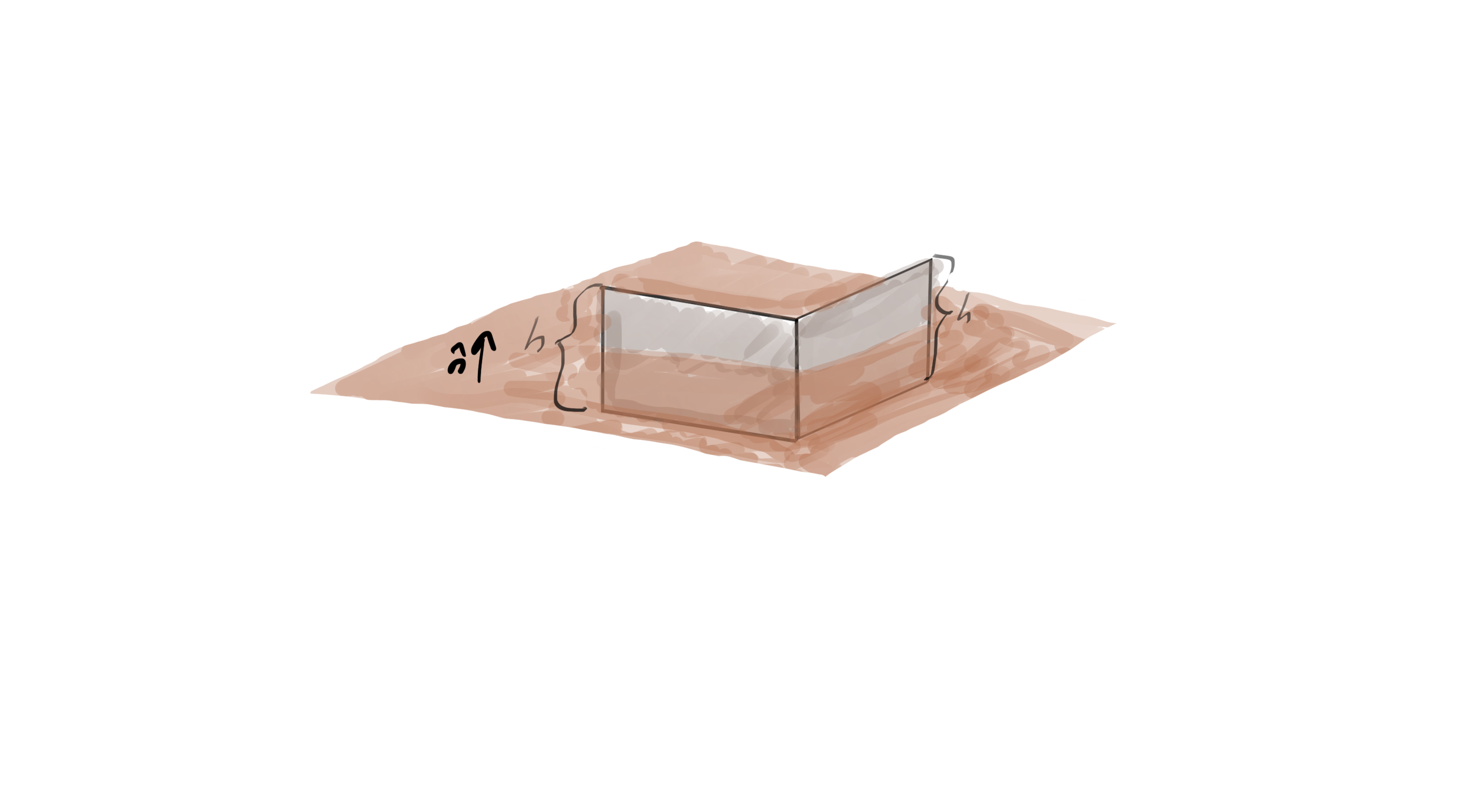
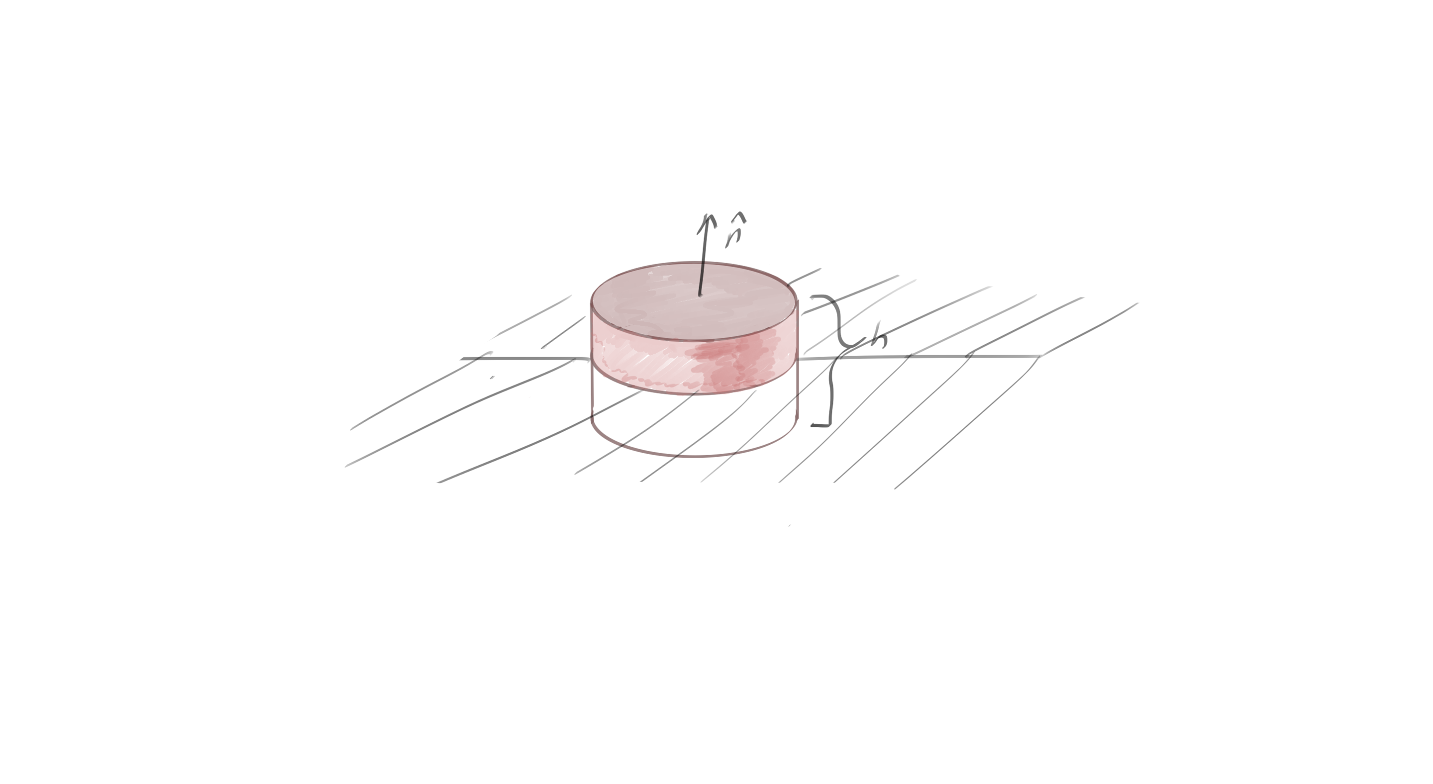
Let \( d^n x’ = dV’ I \), \( d^{n-1} x’ n = dA’ I \), where \( n = n(x’) \) is the outward normal to the area element \( d^{n-1} x’ \). From this point on, lets restrict attention to Euclidean spaces, where \( n^2 = 1 \). In that case
\begin{equation}\label{eqn:gradientGreensFunction:80}
\begin{aligned}
\int_V dV’ G(x,x’) \lrgrad’ F(x’)
&=
\int_V dV’ \lr{G(x,x’) \lgrad’} F(x’)
+
\int_V dV’ G(x,x’) \lr{ \rgrad’ F(x’) } \\
&= \int_{\partial V} dA’ G(x,x’) n F(x’).
\end{aligned}
\end{equation}
Here, the pseudoscalar \( I \) has been factored out by commuting it with \( G \), using \( G I = (-1)^{n-1} I G \), and then pre-multiplication with \( 1/((-1)^{n-1} I ) \).
Each of these integrals can be considered in sequence. A convergence bound is required of the multivector test function \( F(x’) \) on the infinite surface \( \partial V \). Since it’s true that
\begin{equation}\label{eqn:gradientGreensFunction:180}
\Abs{ \int_{\partial V} dA’ G(x,x’) n F(x’) }
\ge
\int_{\partial V} dA’ \Abs{ G(x,x’) n F(x’) },
\end{equation}
then it is sufficient to require that
\begin{equation}\label{eqn:gradientGreensFunction:200}
\lim_{x’ \rightarrow \infty} \Abs{ \frac{x -x’}{\Abs{x – x’}^n} n(x’) F(x’) } \rightarrow 0,
\end{equation}
in order to kill off the surface integral. Evaluating the integral on a hypersphere centred on \( x \) where \( x’ – x = n \Abs{x – x’} \), that is
\begin{equation}\label{eqn:gradientGreensFunction:260}
\lim_{x’ \rightarrow \infty} \frac{ \Abs{F(x’)}}{\Abs{x – x’}^{n-1}} \rightarrow 0.
\end{equation}
Given such a constraint, that leaves
\begin{equation}\label{eqn:gradientGreensFunction:220}
\int_V dV’ \lr{G(x,x’) \lgrad’} F(x’)
=
-\int_V dV’ G(x,x’) \lr{ \rgrad’ F(x’) }.
\end{equation}
The LHS is zero everywhere that \( x \ne x’ \) so it can be restricted to a spherical ball around \( x \), which allows the test function \( F \) to be pulled out of the integral, and a second application of the Fundamental Theorem to be applied.
\begin{equation}\label{eqn:gradientGreensFunction:240}
\begin{aligned}
\int_V dV’ \lr{G(x,x’) \lgrad’} F(x’)
&=
\lim_{\epsilon \rightarrow 0}
\int_{\Abs{x – x’} < \epsilon} dV' \lr{G(x,x') \lgrad'} F(x') \\
&=
\lr{ \lim_{\epsilon \rightarrow 0}
I^{-1} \int_{\Abs{x - x'} < \epsilon} I dV' \lr{G(x,x') \lgrad'}
} F(x) \\
&=
\lr{ \lim_{\epsilon \rightarrow 0}
(-1)^{n-1} I^{-1} \int_{\Abs{x - x'} < \epsilon} G(x,x') d^n x' \lgrad'
} F(x) \\
&=
\lr{ \lim_{\epsilon \rightarrow 0}
(-1)^{n-1} I^{-1} \int_{\Abs{x - x'} = \epsilon} G(x,x') d^{n-1} x'
} F(x) \\
&=
\lr{ \lim_{\epsilon \rightarrow 0}
(-1)^{n-1} I^{-1} \int_{\Abs{x - x'} = \epsilon} G(x,x') dA' I n
} F(x) \\
&=
\lr{ \lim_{\epsilon \rightarrow 0}
\int_{\Abs{x - x'} = \epsilon} dA' G(x,x') n
} F(x) \\
&=
\lr{ \lim_{\epsilon \rightarrow 0}
\int_{\Abs{x - x'} = \epsilon} dA' \frac{\epsilon (-n)}{S_n \epsilon^n} n
} F(x) \\
&=
-\lim_{\epsilon \rightarrow 0}
\frac{F(x)}{S_n \epsilon^{n-1}}
\int_{\Abs{x - x'} = \epsilon} dA' \\
&=
-\lim_{\epsilon \rightarrow 0}
\frac{F(x)}{S_n \epsilon^{n-1}}
S_n \epsilon^{n-1} \\
&=
-F(x).
\end{aligned}
\end{equation}
This essentially calculates the divergence integral around an infinitesimal hypersphere, without assuming that the gradient commutes with the gradient in this infinitesimal region. So, provided the test function is constrained by \ref{eqn:gradientGreensFunction:260}, we have
\begin{equation}\label{eqn:gradientGreensFunction:280}
F(x) = \int_V dV' G(x,x') \lr{ \grad' F(x') }.
\end{equation}
In particular, should we have a first order gradient equation
\begin{equation}\label{eqn:gradientGreensFunction:300}
\spacegrad' F(x') = M(x'),
\end{equation}
the inverse of this equation is given by
\begin{equation}\label{eqn:gradientGreensFunction:320}
\boxed{
F(x) = \int_V dV' G(x,x') M(x').
}
\end{equation}
Note that the sign of the Green's function is explicitly tied to the definition of the convolution integral that is used. This is important since since the conventions for the sign of the Green's function or the parameters in the convolution integral often vary.
What's cool about this result is that it applies not only to gradient equations in Euclidean spaces, but also to multivector (or even just vector) fields \( F \), instead of the usual scalar functions that we usually apply Green's functions to.
Example: Electrostatics
As a check of the sign consider the electrostatics equation
\begin{equation}\label{eqn:gradientGreensFunction:380}
\spacegrad \BE = \frac{\rho}{\epsilon_0},
\end{equation}
for which we have after substitution into \ref{eqn:gradientGreensFunction:320}
\begin{equation}\label{eqn:gradientGreensFunction:400}
\BE(\Bx) = \inv{4 \pi \epsilon_0} \int_V dV’ \frac{\Bx – \Bx’}{\Abs{\Bx – \Bx’}^3} \rho(\Bx’).
\end{equation}
This matches the sign found in a trusted reference such as [2].
Future thought.
Does this Green’s function also work for mixed metric spaces? If so, in such a metric, what does it mean to
calculate the surface area of a unit sphere in a mixed signature space?
References
[1] C. Doran and A.N. Lasenby. Geometric algebra for physicists. Cambridge University Press New York, Cambridge, UK, 1st edition, 2003.
[2] JD Jackson. Classical Electrodynamics. John Wiley and Sons, 2nd edition, 1975.