Month: October 2015

Greetings to new Markham-Unionville conservative rep Bob Saroya.

October 21, 2015 Incoherent ramblings , , , ,

The Honourable Bob Saroya,

Congratulations for your success winning your position in parliament for our district. Unfortunately for you, this means that you are also obligated to represent me. I did not vote for you. I effectively voted none-of-the-above, by voting for the Green Party representative Elvin Kao, knowing full well that he was too inexperienced to be successful. I’m not sad that he was not successful, because his emails expressed a belligerence in foreign policy matters that turned my stomach. He got my vote in the end because he answered my mailed questions, unlike yourself and unlike your like your Liberal running mate Mrs. Jiang. Your Liberal predecessor in Markham Unionville, Mr John McCallum, as a representative, has a 2/5 score for answering correspondence. However, that small non-zero portion of his positive score can really be attributed to his administrative assistant, Mr. Nicholson.

I have a very poor opinion of politics, and politicians, and as my representative, you have an infinitesimal chance of changing that position. Given that you did not answer correspondence sent while running, I do not expect there is much chance of that occurring. What I do expect is to see more voting for increased government when you have the chance. Take bill-C51, the police state bill, tabled by members of Minister Blainey’s hierarchy that effectively gave themselves paychecks and power. Despite knowing that there was a massive objection to this bill, so much that it probably cost the Conservatives their majority this election, it was still forced through. It seems to me that this bill owes its success to the putrid non-democratic policy of the party whip. Because the Liberal leadership was also deluded into thinking there was rational for a new Canadian police state, the average joe like me will slowly start to see how big government in Canada will exploit this to spy on all it’s could-be-terrorist citizens. Welcome to the new Canada, where fear mongering trumps rationality.

I am not surprised that fear mongering is so successful here. We are conditioned to be conformist and patriotic. Our schools are like jails, locked down, with active shooter drills, and require police checks of parent volunteers that discourage involvement of non-school personal in raising the little obedient soldiers who stand for their dose of Oh Canada every morning.

The desired product seems to be unthinking patriots that will be willing to go off to war to bomb the current bad-guy brown people de-jour. Such people are guilty of having been selected as targets by the USA and their North bordered military lackey, but this always occurs in a predictable way. First they are sold or given weapons, then later declared to be enemies. It’s a beautiful scheme to keep the armaments industry going.

What do we not see taught in schools? We don’t see anybody taught to think for themselves. We don’t see basics taught. We are raising a generation of kids that have to use a calculator because they haven’t learned their timetables, and have had the new math shoved down their throats. They won’t be able to multiply the way our generation, our parents, and grandparents learned, but by the time they have been subjected to the matrix method of multiplication, the line crossing method of multiplication, and the array method of multiplication … they will give up. Math will be viewed as too confusing, and we will have a generation of math illiteracy. Our generation has front row seats to watching our first world status get flushed down the toilet.

Ranting aside, I have a couple questions.

1) Should Mr Trudeau follow through with his unlikely promise to repeal parts of bill-C51, imagine that the party whip was given the day off, and you were given the chance to vote in a democratic fashion instead of having to obediently follow the party line like a good Oh Canada trained compliant patriot, how would you vote?

Yes, I know that it is unlikely that the party whip would be given the day off. A more likely scenario is that he/she gets correctly identified as a source of anti-free-speech and anti-democracy, and gets shot by terrorists inspired by Canadian bombing throughout the world.

2) The Quirks and Quarks radio show hosted by Bob McDonald hosted a political debate on science topics. This was a pretty putrid affair, like all politician debates, and the point of the debaters seemed to be to win points for most spin, and least fact.

One point debated seemed to be fact checkable. Opposition members brought up the destruction of one or more Canadian research libraries by the conservative party. The conservative party rep claimed that they were lying, and said that the libraries were not destroyed but digitized to be made available for all. The opposition then predictably claimed that the conservative was also lying.

How many research libraries were destroyed? Where are the digitized copies of all the books available? Was that a 100% digitization, or a partial digitization. If partial, where is the policy used to decide what was destroyed, and are there records showing what was destroyed?

Sincerely,

Peeter Joot
PHY1520H Graduate Quantum Mechanics. Lecture 10: 1D Dirac scattering off potential step. Taught by Prof. Arun Paramekanti

October 20, 2015 phy1520 , ,

[Click here for a PDF of this post with nicer formatting]

Disclaimer

Peeter’s lecture notes from class. These may be incoherent and rough.

These are notes for the UofT course PHY1520, Graduate Quantum Mechanics, taught by Prof. Paramekanti.

Dirac scattering off a potential step

For the non-relativistic case we have

\begin{equation}\label{eqn:qmLecture10:20}
\begin{aligned}
E < V_0 &\Rightarrow T = 0, R = 1 \\ E > V_0 &\Rightarrow T > 0, R < 1.
\end{aligned}
\end{equation}

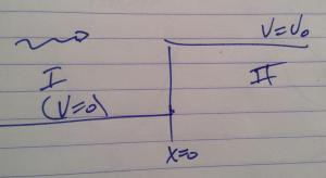
What happens for a relativistic 1D particle?

Referring to fig. 1.

fig. 1. Potential step

fig. 1. Potential step

the region I Hamiltonian is

\begin{equation}\label{eqn:qmLecture10:40}
H =
\begin{bmatrix}
\hat{p} c & m c^2 \\
m c^2 & – \hat{p} c
\end{bmatrix},
\end{equation}

for which the solution is

\begin{equation}\label{eqn:qmLecture10:60}
\Phi = e^{i k_1 x }
\begin{bmatrix}
\cos \theta_1 \\
\sin \theta_1
\end{bmatrix},
\end{equation}

where
\begin{equation}\label{eqn:qmLecture10:80}
\begin{aligned}
\cos 2 \theta_1 &= \frac{ \Hbar c k_1 }{E_{k_1}} \\
\sin 2 \theta_1 &= \frac{ m c^2 }{E_{k_1}} \\
\end{aligned}
\end{equation}

To consider the \( k_1 < 0 \) case, note that

\begin{equation}\label{eqn:qmLecture10:100}
\begin{aligned}
\cos^2 \theta_1 – \sin^2 \theta_1 &= \cos 2 \theta_1 \\
2 \sin\theta_1 \cos\theta_1 &= \sin 2 \theta_1
\end{aligned}
\end{equation}

so after flipping the signs on all the \( k_1 \) terms we find for the reflected wave

\begin{equation}\label{eqn:qmLecture10:120}
\Phi = e^{-i k_1 x}
\begin{bmatrix}
\sin\theta_1 \\
\cos\theta_1
\end{bmatrix}.
\end{equation}

FIXME: this reasoning doesn’t entirely make sense to me. Make sense of this by trying this solution as was done for the form of the incident wave solution.

The region I wave has the form

\begin{equation}\label{eqn:qmLecture10:140}
\Phi_I
=
A e^{i k_1 x}
\begin{bmatrix}
\cos\theta_1 \\
\sin\theta_1 \\
\end{bmatrix}
+
B e^{-i k_1 x}
\begin{bmatrix}
\sin\theta_1 \\
\cos\theta_1 \\
\end{bmatrix}.
\end{equation}

By the time we are done we want to have computed the reflection coefficient

\begin{equation}\label{eqn:qmLecture10:160}
R =
\frac{\Abs{B}^2}{\Abs{A}^2}.
\end{equation}

The region I energy is

\begin{equation}\label{eqn:qmLecture10:180}
E = \sqrt{ \lr{ m c^2}^2 + \lr{ \Hbar c k_1 }^2 }.
\end{equation}

We must have
\begin{equation}\label{eqn:qmLecture10:200}
E
=
\sqrt{ \lr{ m c^2}^2 + \lr{ \Hbar c k_2 }^2 } + V_0
=
\sqrt{ \lr{ m c^2}^2 + \lr{ \Hbar c k_1 }^2 },
\end{equation}

so

\begin{equation}\label{eqn:qmLecture10:220}
\begin{aligned}
\lr{ \Hbar c k_2 }^2
&=
\lr{ E – V_0 }^2 – \lr{ m c^2}^2 \\
&=
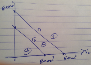
\underbrace{\lr{ E – V_0 + m c }}_{r_1}\underbrace{\lr{ E – V_0 – m c }}_{r_2}.
\end{aligned}
\end{equation}

The \( r_1 \) and \( r_2 \) branches are sketched in fig. 2.

fig. 2. Energy signs

fig. 2. Energy signs

For low energies, we have a set of potentials for which we will have propagation, despite having a potential barrier. For still higher values of the potential barrier the product \( r_1 r_2 \) will be negative, so the solutions will be decaying. Finally, for even higher energies, there will again be propagation.

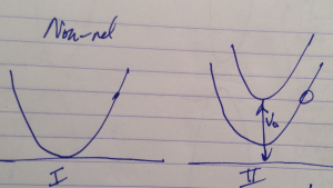
The non-relativistic case is sketched in fig. 3.

fig. 3. Effects of increasing potential for non-relativistic case

fig. 3. Effects of increasing potential for non-relativistic case

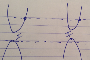
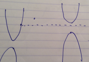
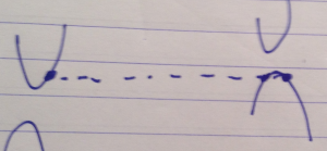
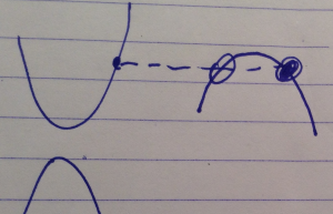
For the relativistic case we must consider three different cases, sketched in fig 4, fig 5, and fig 6 respectively. For the low potential energy, a particle with positive group velocity (what we’ve called right moving) can be matched to an equal energy portion of the potential shifted parabola in region II. This is a case where we have transmission, but no antiparticle creation. There will be an energy region where the region II wave function has only a dissipative term, since there is no region of either of the region II parabolic branches available at the incident energy. When the potential is shifted still higher so that \( V_0 > E + m c^2 \), a positive group velocity in region I with a given energy can be matched to an antiparticle branch in the region II parabolic energy curve.

lecture10Fig4a

Fig 4. Low potential energy

lecture10Fig4b

fig. 5. High enough potential energy for no propagation

lecture10Fig4c

fig 6. High potential energy


Boundary value conditions

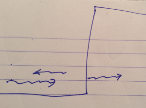
We want to ensure that the current across the barrier is conserved (no particles are lost), as sketched in fig. 7.


fig. 7. Transmitted, reflected and incident components.

fig. 7. Transmitted, reflected and incident components.

Recall that given a wave function

\begin{equation}\label{eqn:qmLecture10:240}
\Psi =
\begin{bmatrix}
\psi_1 \\
\psi_2
\end{bmatrix},
\end{equation}

the density and currents are respectively

\begin{equation}\label{eqn:qmLecture10:260}
\begin{aligned}
\rho &= \psi_1^\conj \psi_1 + \psi_2^\conj \psi_2 \\
j &= \psi_1^\conj \psi_1 – \psi_2^\conj \psi_2
\end{aligned}
\end{equation}

Matching boundary value conditions requires

  1. For both the relativistic and non-relativistic cases we must have\begin{equation}\label{eqn:qmLecture10:280}
    \Psi_{\textrm{L}} = \Psi_{\textrm{R}}, \qquad \mbox{at \( x = 0 \).}
    \end{equation}
  2. For the non-relativistic case we want
    \begin{equation}\label{eqn:qmLecture10:300}
    \int_{-\epsilon}^\epsilon -\frac{\Hbar^2}{2m} \PDSq{x}{\Psi} =
    {\int_{-\epsilon}^\epsilon \lr{ E – V(x) } \Psi(x)}.
    \end{equation}The RHS integral is zero, so

    \begin{equation}\label{eqn:qmLecture10:320}
    -\frac{\Hbar^2}{2m} \lr{ \evalbar{\PD{x}{\Psi}}{{\textrm{R}}} – \evalbar{\PD{x}{\Psi}}{{\textrm{L}}} } = 0.
    \end{equation}

    We have to match

    For the relativistic case

    \begin{equation}\label{eqn:qmLecture10:460}
    -i \Hbar \sigma_z \int_{-\epsilon}^\epsilon \PD{x}{\Psi} +
    {m c^2 \sigma_x \int_{-\epsilon}^\epsilon \psi}
    =
    {\int_{-\epsilon}^\epsilon \lr{ E – V_0 } \psi},
    \end{equation}

the second two integrals are wiped out, so

\begin{equation}\label{eqn:qmLecture10:340}
-i \Hbar c \sigma_z \lr{ \psi(\epsilon) – \psi(-\epsilon) }
=
-i \Hbar c \sigma_z \lr{ \psi_{\textrm{R}} – \psi_{\textrm{L}} }.
\end{equation}

so we must match

\begin{equation}\label{eqn:qmLecture10:360}
\sigma_z \psi_{\textrm{R}} = \sigma_z \psi_{\textrm{L}} .
\end{equation}

It appears that things are simpler, because we only have to match the wave function values at the boundary, and don’t have to match the derivatives too. However, we have a two component wave function, so there are still two tasks.

Solving the system

Let’s look for a solution for the \( E + m c^2 > V_0 \) case on the right branch, as sketched in fig. 8.


fig. 8. High potential region. Anti-particle transmission.

fig. 8. High potential region. Anti-particle transmission.

While the right branch in this case is left going, this might work out since that is an antiparticle. We could try both.

Try

\begin{equation}\label{eqn:qmLecture10:480}
\Psi_{II} = D e^{i k_2 x}
\begin{bmatrix}
-\sin\theta_2 \\
\cos\theta_2
\end{bmatrix}.
\end{equation}

This is justified by

\begin{equation}\label{eqn:qmLecture10:500}
+E \rightarrow
\begin{bmatrix}
\cos\theta \\
\sin\theta
\end{bmatrix},
\end{equation}

so

\begin{equation}\label{eqn:qmLecture10:520}
-E \rightarrow
\begin{bmatrix}
-\sin\theta \\
\cos\theta \\
\end{bmatrix}
\end{equation}

At \( x = 0 \) the exponentials vanish, so equating the waves at that point means

\begin{equation}\label{eqn:qmLecture10:380}
\begin{bmatrix}
\cos\theta_1 \\
\sin\theta_1 \\
\end{bmatrix}
+
\frac{B}{A}
\begin{bmatrix}
\sin\theta_1 \\
\cos\theta_1 \\
\end{bmatrix}
=
\frac{D}{A}
\begin{bmatrix}
-\sin\theta_2 \\
\cos\theta_2
\end{bmatrix}.
\end{equation}

Solving this yields

\begin{equation}\label{eqn:qmLecture10:400}
\frac{B}{A} = – \frac{\cos(\theta_1 – \theta_2)}{\sin(\theta_1 + \theta_2)}.
\end{equation}

This yields

\begin{equation}\label{eqn:qmLecture10:420}
\boxed{
R = \frac{1 + \cos( 2 \theta_1 – 2 \theta_2) }{1 – \cos( 2 \theta_1 – 2 \theta_2)}.
}
\end{equation}

As \( V_0 \rightarrow \infty \) this simplifies to

\begin{equation}\label{eqn:qmLecture10:440}
R = \frac{ E – \sqrt{ E^2 – \lr{ m c^2 }^2 } }{ E + \sqrt{ E^2 – \lr{ m c^2 }^2 } }.
\end{equation}

Filling in the details for these results part of problem set 4.

Second update of aggregate notes for phy1520, Graduate Quantum Mechanics

October 20, 2015 phy1520 , , , , , , , , , , , ,

I’ve posted a second update of my aggregate notes for PHY1520H Graduate Quantum Mechanics, taught by Prof. Arun Paramekanti. In addition to what was noted previously, this contains lecture notes up to lecture 9, my ungraded solutions for the second problem set, and some additional worked practise problems.

Most of the content was posted individually in the following locations, but those original documents will not be maintained individually any further.

Plane wave ground state expectation for SHO

October 18, 2015 phy1520 , , , , , , , , , , ,

[Click here for a PDF of this post with nicer formatting]

Problem [1] 2.18 is, for a 1D SHO, show that

\begin{equation}\label{eqn:exponentialExpectationGroundState:20}
\bra{0} e^{i k x} \ket{0} = \exp\lr{ -k^2 \bra{0} x^2 \ket{0}/2 }.
\end{equation}

Despite the simple appearance of this problem, I found this quite involved to show. To do so, start with a series expansion of the expectation

\begin{equation}\label{eqn:exponentialExpectationGroundState:40}
\bra{0} e^{i k x} \ket{0}
=
\sum_{m=0}^\infty \frac{(i k)^m}{m!} \bra{0} x^m \ket{0}.
\end{equation}

Let

\begin{equation}\label{eqn:exponentialExpectationGroundState:60}
X = \lr{ a + a^\dagger },
\end{equation}

so that

\begin{equation}\label{eqn:exponentialExpectationGroundState:80}
x
= \sqrt{\frac{\Hbar}{2 \omega m}} X
= \frac{x_0}{\sqrt{2}} X.
\end{equation}

Consider the first few values of \( \bra{0} X^n \ket{0} \)

\begin{equation}\label{eqn:exponentialExpectationGroundState:100}
\begin{aligned}
\bra{0} X \ket{0}
&=
\bra{0} \lr{ a + a^\dagger } \ket{0} \\
&=
\braket{0}{1} \\
&=
0,
\end{aligned}
\end{equation}

\begin{equation}\label{eqn:exponentialExpectationGroundState:120}
\begin{aligned}
\bra{0} X^2 \ket{0}
&=
\bra{0} \lr{ a + a^\dagger }^2 \ket{0} \\
&=
\braket{1}{1} \\
&=
1,
\end{aligned}
\end{equation}

\begin{equation}\label{eqn:exponentialExpectationGroundState:140}
\begin{aligned}
\bra{0} X^3 \ket{0}
&=
\bra{0} \lr{ a + a^\dagger }^3 \ket{0} \\
&=
\bra{1} \lr{ \sqrt{2} \ket{2} + \ket{0} } \\
&=
0.
\end{aligned}
\end{equation}

Whenever the power \( n \) in \( X^n \) is even, the braket can be split into a bra that has only contributions from odd eigenstates and a ket with even eigenstates. We conclude that \( \bra{0} X^n \ket{0} = 0 \) when \( n \) is odd.

Noting that \( \bra{0} x^2 \ket{0} = \ifrac{x_0^2}{2} \), this leaves

\begin{equation}\label{eqn:exponentialExpectationGroundState:160}
\begin{aligned}
\bra{0} e^{i k x} \ket{0}
&=
\sum_{m=0}^\infty \frac{(i k)^{2 m}}{(2 m)!} \bra{0} x^{2m} \ket{0} \\
&=
\sum_{m=0}^\infty \frac{(i k)^{2 m}}{(2 m)!} \lr{ \frac{x_0^2}{2} }^m \bra{0} X^{2m} \ket{0} \\
&=
\sum_{m=0}^\infty \frac{1}{(2 m)!} \lr{ -k^2 \bra{0} x^2 \ket{0} }^m \bra{0} X^{2m} \ket{0}.
\end{aligned}
\end{equation}

This problem is now reduced to showing that

\begin{equation}\label{eqn:exponentialExpectationGroundState:180}
\frac{1}{(2 m)!} \bra{0} X^{2m} \ket{0} = \inv{m! 2^m},
\end{equation}

or

\begin{equation}\label{eqn:exponentialExpectationGroundState:200}
\begin{aligned}
\bra{0} X^{2m} \ket{0}
&= \frac{(2m)!}{m! 2^m} \\
&= \frac{ (2m)(2m-1)(2m-2) \cdots (2)(1) }{2^m m!} \\
&= \frac{ 2^m (m)(2m-1)(m-1)(2m-3)(m-2) \cdots (2)(3)(1)(1) }{2^m m!} \\
&= (2m-1)!!,
\end{aligned}
\end{equation}

where \( n!! = n(n-2)(n-4)\cdots \).

It looks like \( \bra{0} X^{2m} \ket{0} \) can be expanded by inserting an identity operator and proceeding recursively, like

\begin{equation}\label{eqn:exponentialExpectationGroundState:220}
\begin{aligned}
\bra{0} X^{2m} \ket{0}
&=
\bra{0} X^2 \lr{ \sum_{n=0}^\infty \ket{n}\bra{n} } X^{2m-2} \ket{0} \\
&=
\bra{0} X^2 \lr{ \ket{0}\bra{0} + \ket{2}\bra{2} } X^{2m-2} \ket{0} \\
&=
\bra{0} X^{2m-2} \ket{0} + \bra{0} X^2 \ket{2} \bra{2} X^{2m-2} \ket{0}.
\end{aligned}
\end{equation}

This has made use of the observation that \( \bra{0} X^2 \ket{n} = 0 \) for all \( n \ne 0,2 \). The remaining term includes the factor

\begin{equation}\label{eqn:exponentialExpectationGroundState:240}
\begin{aligned}
\bra{0} X^2 \ket{2}
&=
\bra{0} \lr{a + a^\dagger}^2 \ket{2} \\
&=
\lr{ \bra{0} + \sqrt{2} \bra{2} } \ket{2} \\
&=
\sqrt{2},
\end{aligned}
\end{equation}

Since \( \sqrt{2} \ket{2} = \lr{a^\dagger}^2 \ket{0} \), the expectation of interest can be written

\begin{equation}\label{eqn:exponentialExpectationGroundState:260}
\bra{0} X^{2m} \ket{0}
=
\bra{0} X^{2m-2} \ket{0} + \bra{0} a^2 X^{2m-2} \ket{0}.
\end{equation}

How do we expand the second term. Let’s look at how \( a \) and \( X \) commute

\begin{equation}\label{eqn:exponentialExpectationGroundState:280}
\begin{aligned}
a X
&=
\antisymmetric{a}{X} + X a \\
&=
\antisymmetric{a}{a + a^\dagger} + X a \\
&=
\antisymmetric{a}{a^\dagger} + X a \\
&=
1 + X a,
\end{aligned}
\end{equation}

\begin{equation}\label{eqn:exponentialExpectationGroundState:300}
\begin{aligned}
a^2 X
&=
a \lr{ a X } \\
&=
a \lr{ 1 + X a } \\
&=
a + a X a \\
&=
a + \lr{ 1 + X a } a \\
&=
2 a + X a^2.
\end{aligned}
\end{equation}

Proceeding to expand \( a^2 X^n \) we find
\begin{equation}\label{eqn:exponentialExpectationGroundState:320}
\begin{aligned}
a^2 X^3 &= 6 X + 6 X^2 a + X^3 a^2 \\
a^2 X^4 &= 12 X^2 + 8 X^3 a + X^4 a^2 \\
a^2 X^5 &= 20 X^3 + 10 X^4 a + X^5 a^2 \\
a^2 X^6 &= 30 X^4 + 12 X^5 a + X^6 a^2.
\end{aligned}
\end{equation}

It appears that we have
\begin{equation}\label{eqn:exponentialExpectationGroundState:340}
\antisymmetric{a^2 X^n}{X^n a^2} = \beta_n X^{n-2} + 2 n X^{n-1} a,
\end{equation}

where

\begin{equation}\label{eqn:exponentialExpectationGroundState:360}
\beta_n = \beta_{n-1} + 2 (n-1),
\end{equation}

and \( \beta_2 = 2 \). Some goofing around shows that \( \beta_n = n(n-1) \), so the induction hypothesis is

\begin{equation}\label{eqn:exponentialExpectationGroundState:380}
\antisymmetric{a^2 X^n}{X^n a^2} = n(n-1) X^{n-2} + 2 n X^{n-1} a.
\end{equation}

Let’s check the induction
\begin{equation}\label{eqn:exponentialExpectationGroundState:400}
\begin{aligned}
a^2 X^{n+1}
&=
a^2 X^{n} X \\
&=
\lr{ n(n-1) X^{n-2} + 2 n X^{n-1} a + X^n a^2 } X \\
&=
n(n-1) X^{n-1} + 2 n X^{n-1} a X + X^n a^2 X \\
&=
n(n-1) X^{n-1} + 2 n X^{n-1} \lr{ 1 + X a } + X^n \lr{ 2 a + X a^2 } \\
&=
n(n-1) X^{n-1} + 2 n X^{n-1} + 2 n X^{n} a
+ 2 X^n a
+ X^{n+1} a^2 \\
&=
X^{n+1} a^2 + (2 + 2 n) X^{n} a + \lr{ 2 n + n(n-1) } X^{n-1} \\
&=
X^{n+1} a^2 + 2(n + 1) X^{n} a + (n+1) n X^{n-1},
\end{aligned}
\end{equation}

which concludes the induction, giving

\begin{equation}\label{eqn:exponentialExpectationGroundState:420}
\bra{ 0 } a^2 X^{n} \ket{0 } = n(n-1) \bra{0} X^{n-2} \ket{0},
\end{equation}

and

\begin{equation}\label{eqn:exponentialExpectationGroundState:440}
\bra{0} X^{2m} \ket{0}
=
\bra{0} X^{2m-2} \ket{0} + (2m-2)(2m-3) \bra{0} X^{2m-4} \ket{0}.
\end{equation}

Let

\begin{equation}\label{eqn:exponentialExpectationGroundState:460}
\sigma_{n} = \bra{0} X^n \ket{0},
\end{equation}

so that the recurrence relation, for \( 2n \ge 4 \) is

\begin{equation}\label{eqn:exponentialExpectationGroundState:480}
\sigma_{2n} = \sigma_{2n -2} + (2n-2)(2n-3) \sigma_{2n -4}
\end{equation}

We want to show that this simplifies to

\begin{equation}\label{eqn:exponentialExpectationGroundState:500}
\sigma_{2n} = (2n-1)!!
\end{equation}

The first values are

\begin{equation}\label{eqn:exponentialExpectationGroundState:540}
\sigma_0 = \bra{0} X^0 \ket{0} = 1
\end{equation}
\begin{equation}\label{eqn:exponentialExpectationGroundState:560}
\sigma_2 = \bra{0} X^2 \ket{0} = 1
\end{equation}

which gives us the right result for the first term in the induction

\begin{equation}\label{eqn:exponentialExpectationGroundState:580}
\begin{aligned}
\sigma_4
&= \sigma_2 + 2 \times 1 \times \sigma_0 \\
&= 1 + 2 \\
&= 3!!
\end{aligned}
\end{equation}

For the general induction term, consider

\begin{equation}\label{eqn:exponentialExpectationGroundState:600}
\begin{aligned}
\sigma_{2n + 2}
&= \sigma_{2n} + 2 n (2n – 1) \sigma_{2n -2} \\
&= (2n-1)!! + 2n ( 2n – 1) (2n -3)!! \\
&= (2n + 1) (2n -1)!! \\
&= (2n + 1)!!,
\end{aligned}
\end{equation}

which completes the final induction. That was also the last thing required to complete the proof, so we are done!

References

[1] Jun John Sakurai and Jim J Napolitano. Modern quantum mechanics. Pearson Higher Ed, 2014.

PHY1520H Graduate Quantum Mechanics. Lecture 7: Aharonov-Bohm effect and Landau levels. Taught by Prof. Arun Paramekanti

October 16, 2015 phy1520 , , ,

[Click here for a PDF of this post with nicer formatting]

Disclaimer

Peeter’s lecture notes from class. These may be incoherent and rough.

These are notes for the UofT course PHY1520, Graduate Quantum Mechanics, taught by Prof. Paramekanti, covering [1] chap. 2 content.

problem set note.

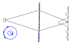
In the problem set we’ll look at interference patterns for two slit electron interference like that of fig. 1, where a magnetic whisker that introduces flux is added to the configuration.

fig. 1. Two slit interference with magnetic whisker

fig. 1. Two slit interference with magnetic whisker

Aharonov-Bohm effect (cont.)

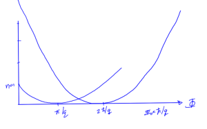
fig. 2. Energy vs flux

fig. 2. Energy vs flux

Why do we have the zeros at integral multiples of \( h/q \)? Consider a particle in a circular trajectory as sketched in fig. 3

fig. 3. Circular trajectory

fig. 3. Circular trajectory

FIXME: Prof mentioned:

\begin{equation}\label{eqn:qmLecture7:20}
\phi_{\textrm{loop}} = q \frac{ h p/ q }{\Hbar} = 2 \pi p
\end{equation}

… I’m not sure what that was about now.

In classical mechanics we have

\begin{equation}\label{eqn:qmLecture7:40}
\oint p dq
\end{equation}

The integral zero points are related to such a loop, but the \( q \BA \) portion of the momentum \( \Bp – q \BA \) needs to be considered.

Superconductors

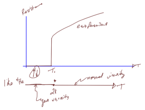
After cooling some materials sufficiently, superconductivity, a complete lack of resistance to electrical flow can be observed. A resistivity vs temperature plot of such a material is sketched in fig. 4.

fig. 4. Superconductivity with comparison to superfluidity

fig. 4. Superconductivity with comparison to superfluidity

Just like \ce{He^4} can undergo Bose condensation, superconductivity can be explained by a hybrid Bosonic state where electrons are paired into one state containing integral spin.

The Little-Parks experiment puts a superconducting ring around a magnetic whisker as sketched in fig. 6.

fig. 6. Little-Parks superconducting ring

fig. 6. Little-Parks superconducting ring

This experiment shows that the effective charge of the circulating charge was \( 2 e \), validating the concept of Cooper-pairing, the Bosonic combination (integral spin) of electrons in superconduction.

Motion around magnetic field

\begin{equation}\label{eqn:qmLecture7:140}
\omega_{\textrm{c}} = \frac{e B}{m}
\end{equation}

We work with what is now called the Landau gauge

\begin{equation}\label{eqn:qmLecture7:60}
\BA = \lr{ 0, B x, 0 }
\end{equation}

This gives

\begin{equation}\label{eqn:qmLecture7:80}
\begin{aligned}
\BB
&= \spacegrad \cross \BA \\
&= \lr{ \partial_x A_y – \partial_y A_x } \zcap \\
&= B \zcap.
\end{aligned}
\end{equation}

An alternate gauge choice, the symmetric gauge, is

\begin{equation}\label{eqn:qmLecture7:100}
\BA = \lr{ -\frac{B y}{2}, \frac{B x}{2}, 0 },
\end{equation}

that also has the same magnetic field

\begin{equation}\label{eqn:qmLecture7:120}
\begin{aligned}
\BB
&= \spacegrad \BA \\
&= \lr{ \partial_x A_y – \partial_y A_x } \zcap \\
&= \lr{ \frac{B}{2} – \lr{ – \frac{B}{2} } } \zcap \\
&= B \zcap.
\end{aligned}
\end{equation}

We expect the physics for each to have the same results, although the wave functions in one gauge may be more complicated than in the other.

Our Hamiltonian is

\begin{equation}\label{eqn:qmLecture7:160}
\begin{aligned}
H
&= \inv{2 m} \lr{ \Bp – e \BA }^2 \\
&= \inv{2 m} \hat{p}_x^2 + \inv{2 m} \lr{ \hat{p}_y – e B \xhat }^2
\end{aligned}
\end{equation}

We can solve after noting that

\begin{equation}\label{eqn:qmLecture7:180}
\antisymmetric{\hat{p}_y}{H} = 0
\end{equation}

means that

\begin{equation}\label{eqn:qmLecture7:200}
\Psi(x,y) = e^{i k_y y} \phi(x)
\end{equation}

The eigensystem

\begin{equation}\label{eqn:qmLecture7:220}
H \psi(x, y) = E \phi(x, y) ,
\end{equation}

becomes

\begin{equation}\label{eqn:qmLecture7:240}
\lr{ \inv{2 m} \hat{p}_x^2 + \inv{2 m} \lr{ \Hbar k_y – e B \xhat}^2 } \phi(x)
= E \phi(x).
\end{equation}

This reduced Hamiltonian can be rewritten as

\begin{equation}\label{eqn:qmLecture7:320}
H_x
= \inv{2 m} p_x^2 + \inv{2 m} e^2 B^2 \lr{ \xhat – \frac{\Hbar k_y}{e B} }^2
\equiv \inv{2 m} p_x^2 + \inv{2} m \omega^2 \lr{ \xhat – x_0 }^2
\end{equation}

where

\begin{equation}\label{eqn:qmLecture7:260}
\inv{2 m} e^2 B^2 = \inv{2} m \omega^2,
\end{equation}

or
\begin{equation}\label{eqn:qmLecture7:280}
\omega = \frac{ e B}{m} \equiv \omega_{\textrm{c}}.
\end{equation}

and

\begin{equation}\label{eqn:qmLecture7:300}
x_0 = \frac{\Hbar}{k_y}{e B}.
\end{equation}

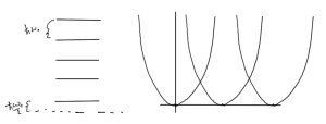
But what is this \( x_0 \)? Because \( k_y \) is not really specified in this problem, we can consider that we have a zero point energy for every \( k_y \), but the oscillator position is shifted for every such value of \( k_y \). For each set of energy levels fig. 8 we can consider that there is a different zero point energy for each possible \( k_y \).

fig. 8. Energy levels, and Energy vs flux

fig. 8. Energy levels, and Energy vs flux

This is an infinitely degenerate system with an infinite number of states for any given energy level.

This tells us that there is a problem, and have to reconsider the assumption that any \( k_y \) is acceptable.

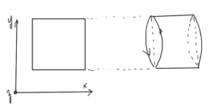
To resolve this we can introduce periodic boundary conditions, imagining that a square is rotated in space forming a cylinder as sketched in fig. 9.

fig. 9. Landau degeneracy region

fig. 9. Landau degeneracy region

Requiring quantized momentum

\begin{equation}\label{eqn:qmLecture7:340}
k_y L_y = 2 \pi n,
\end{equation}

or

\begin{equation}\label{eqn:qmLecture7:360}
k_y = \frac{2 \pi n}{L_y}, \qquad n \in \mathbb{Z},
\end{equation}

gives

\begin{equation}\label{eqn:qmLecture7:380}
x_0(n) = \frac{\Hbar}{e B} \frac{ 2 \pi n}{L_y},
\end{equation}

with \( x_0 \le L_x \). The range is thus restricted to

\begin{equation}\label{eqn:qmLecture7:400}
\frac{\Hbar}{e B} \frac{ 2 \pi n_{\textrm{max}}}{L_y} = L_x,
\end{equation}

or

\begin{equation}\label{eqn:qmLecture7:420}
n_{\textrm{max}} = \underbrace{L_x L_y}_{\text{area}} \frac{ e B }{2 \pi \Hbar }
\end{equation}

That is

\begin{equation}\label{eqn:qmLecture7:440}
\begin{aligned}
n_{\textrm{max}}
&= \frac{\Phi_{\textrm{total}}}{h/e} \\
&= \frac{\Phi_{\textrm{total}}}{\Phi_0}.
\end{aligned}
\end{equation}

Attempting to measure Hall-effect systems, it was found that the Hall conductivity was quantized like

\begin{equation}\label{eqn:qmLecture7:460}
\sigma_{x y} = p \frac{e^2}{h}.
\end{equation}

This quantization is explained by these Landau levels, and this experimental apparatus provides one of the more accurate ways to measure the fine structure constant.

References

[1] Jun John Sakurai and Jim J Napolitano. Modern quantum mechanics. Pearson Higher Ed, 2014.