[Click here for a PDF of this post with nicer formatting]
Disclaimer
Peeter’s lecture notes from class. These may be incoherent and rough.
These are notes for the UofT course PHY1520, Graduate Quantum Mechanics, taught by Prof. Paramekanti, covering \textchapref{{4}} [1] content.
Symmetry in classical mechanics
In a classical context considering a Hamiltonian
\begin{equation}\label{eqn:qmLecture11:20}
H(q_i, p_i),
\end{equation}
a symmetry means that certain \( q_i \) don’t appear. In that case the rate of change of one of the generalized momenta is zero
\begin{equation}\label{eqn:qmLecture11:40}
\ddt{p_k} = – \PD{q_k}{H} = 0,
\end{equation}
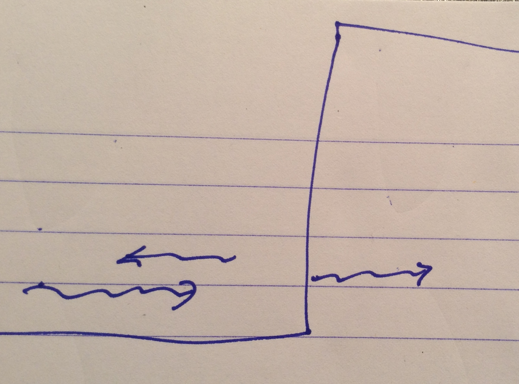
so \( p_k \) is a constant of motion. This simplifies the problem by reducing the number of degrees of freedom. Another aspect of such a symmetry is that it \underline{relates trajectories}. For example, assuming a rotational symmetry as in fig. 1.
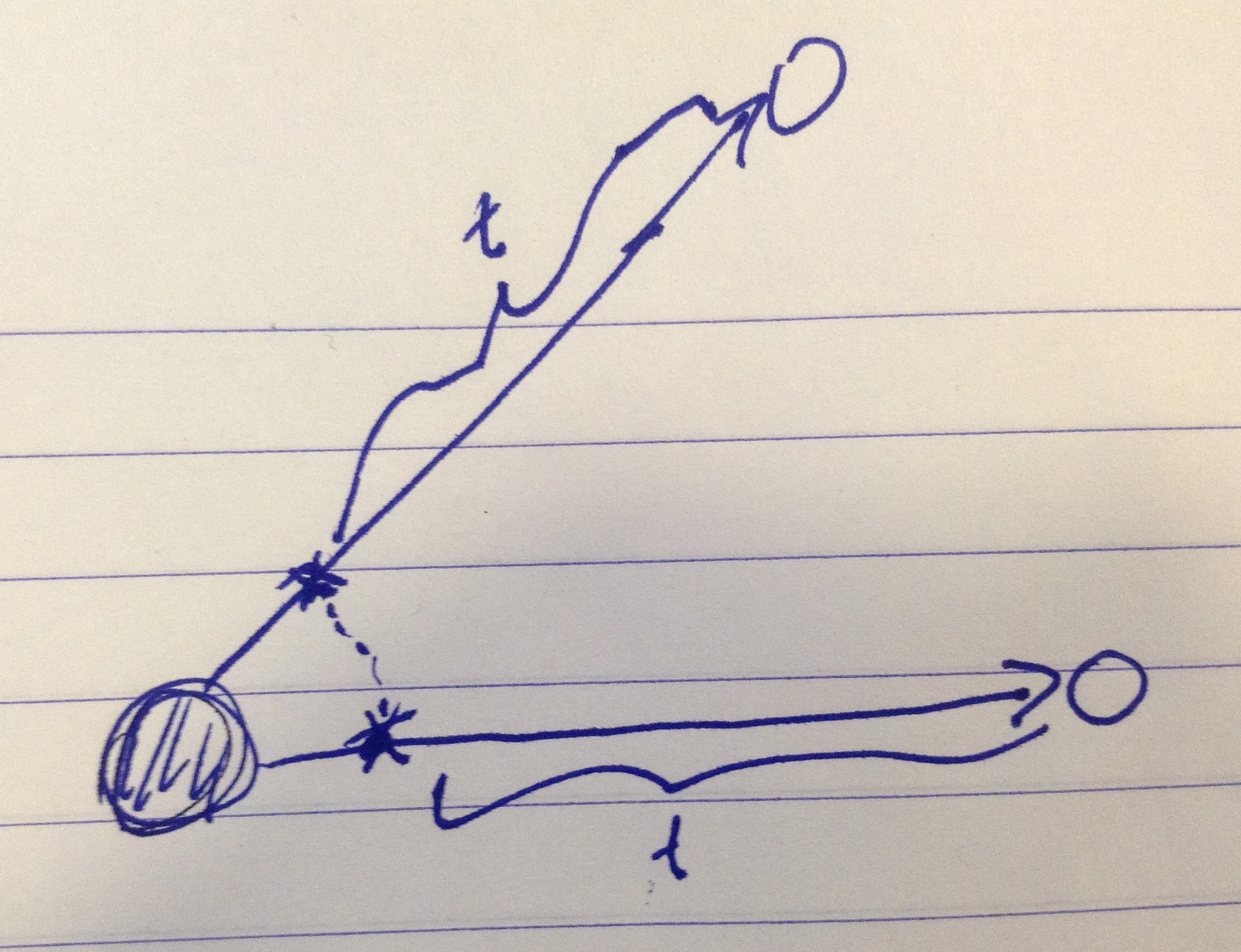
fig. 1. Trajectory under rotational symmetry
the trajectory of a particle after rotation is related by rotation to the trajectory of the unrotated particle.
Symmetry in quantum mechanics
Suppose that we have a symmetry operation that takes states from
\begin{equation}\label{eqn:qmLecture11:60}
\ket{\psi} \rightarrow \ket{U \psi}
\end{equation}
\begin{equation}\label{eqn:qmLecture11:80}
\ket{\phi} \rightarrow \ket{U \phi},
\end{equation}
we expect that
\begin{equation}\label{eqn:qmLecture11:100}
\Abs{\braket{ \psi}{\phi} }^2 = \Abs{\braket{ U\psi}{ U\phi} }^2.
\end{equation}
This won’t hold true for a general operator. Two cases where this does hold true is when
- \( \braket{\psi}{\phi} = \braket{ U\psi}{ U\phi} \). Here \( U \) is unitary, and the equivalence follows from
\begin{equation}\label{eqn:qmLecture11:120}
\braket{ U\psi}{ U\phi} = \bra{ \psi} U^\dagger U { \phi} = \bra{ \psi} 1 { \phi} = \braket{\psi}{\phi}.
\end{equation} - \( \braket{\psi}{\phi} = \braket{ U\psi}{ U\phi}^\conj \). Here \( U \) is anti-unitary.
Unitary case
If an “observable” is not changed by a unitary operation representing a symmetry we must have
\begin{equation}\label{eqn:qmLecture11:140}
\bra{\psi} \hat{A} \ket{\psi}
\rightarrow
\bra{U \psi} \hat{A} \ket{U \psi}
=
\bra{\psi} U^\dagger \hat{A} U \ket{\psi},
\end{equation}
so
\begin{equation}\label{eqn:qmLecture11:160}
U^\dagger \hat{A} U = \hat{A},
\end{equation}
or
\begin{equation}\label{eqn:qmLecture11:180}
\boxed{
\hat{A} U = U \hat{A}.
}
\end{equation}
An observable that is unchanged by a unitary symmetry commutes \( \antisymmetric{\hat{A}}{U} \) with the operator \( U \) for that transformation.
Symmetries of the Hamiltonian
Given
\begin{equation}\label{eqn:qmLecture11:200}
\antisymmetric{H}{U} = 0,
\end{equation}
\( H \) is invariant.
Given
\begin{equation}\label{eqn:qmLecture11:220}
H \ket{\phi_n} = \epsilon_n \ket{\phi_n} .
\end{equation}
\begin{equation}\label{eqn:qmLecture11:240}
\begin{aligned}
U H \ket{\phi_n}
&= H U \ket{\phi_n} \\
&= \epsilon_n U \ket{\phi_n}
\end{aligned}
\end{equation}
Such a state
\begin{equation}\label{eqn:qmLecture11:260}
\ket{\psi_n} = U \ket{\phi_n}
\end{equation}
is also an eigenstate with the \underline{same} energy.
Suppose this process is repeated, finding other states
\begin{equation}\label{eqn:qmLecture11:280}
U \ket{\psi_n} = \ket{\chi_n}
\end{equation}
\begin{equation}\label{eqn:qmLecture11:300}
U \ket{\chi_n} = \ket{\alpha_n}
\end{equation}
Because such a transformation only generates states with the initial energy, this process cannot continue forever. At some point this process will enumerate a fixed size set of states. These states can be orthonormalized.
We can say that symmetry operations are generators of a \underlineAndIndex{group}. For a set of symmetry operations we can
-
Form products that lie in a closed set
\begin{equation}\label{eqn:qmLecture11:320}
U_1 U_2 = U_3
\end{equation} - can define an inverse
\begin{equation}\label{eqn:qmLecture11:340}
U \leftrightarrow U^{-1}.
\end{equation} - obeys associative rules for multiplication
\begin{equation}\label{eqn:qmLecture11:360}
U_1 ( U_2 U_3 ) = (U_1 U_2) U_3.
\end{equation} - has an identity operation.
When \( H \) has a symmetry, then degenerate eigenstates form \underlineAndIndex{irreducible} representations (which cannot be further block diagonalized).
Some simple examples
Example: Inversion.
{example:qmLecture11:1}
Given a state and a parity operation \( \hat{\Pi} \), with the transformation
\begin{equation}\label{eqn:qmLecture11:380}
\ket{\psi} \rightarrow \hat{\Pi} \ket{\psi}
\end{equation}
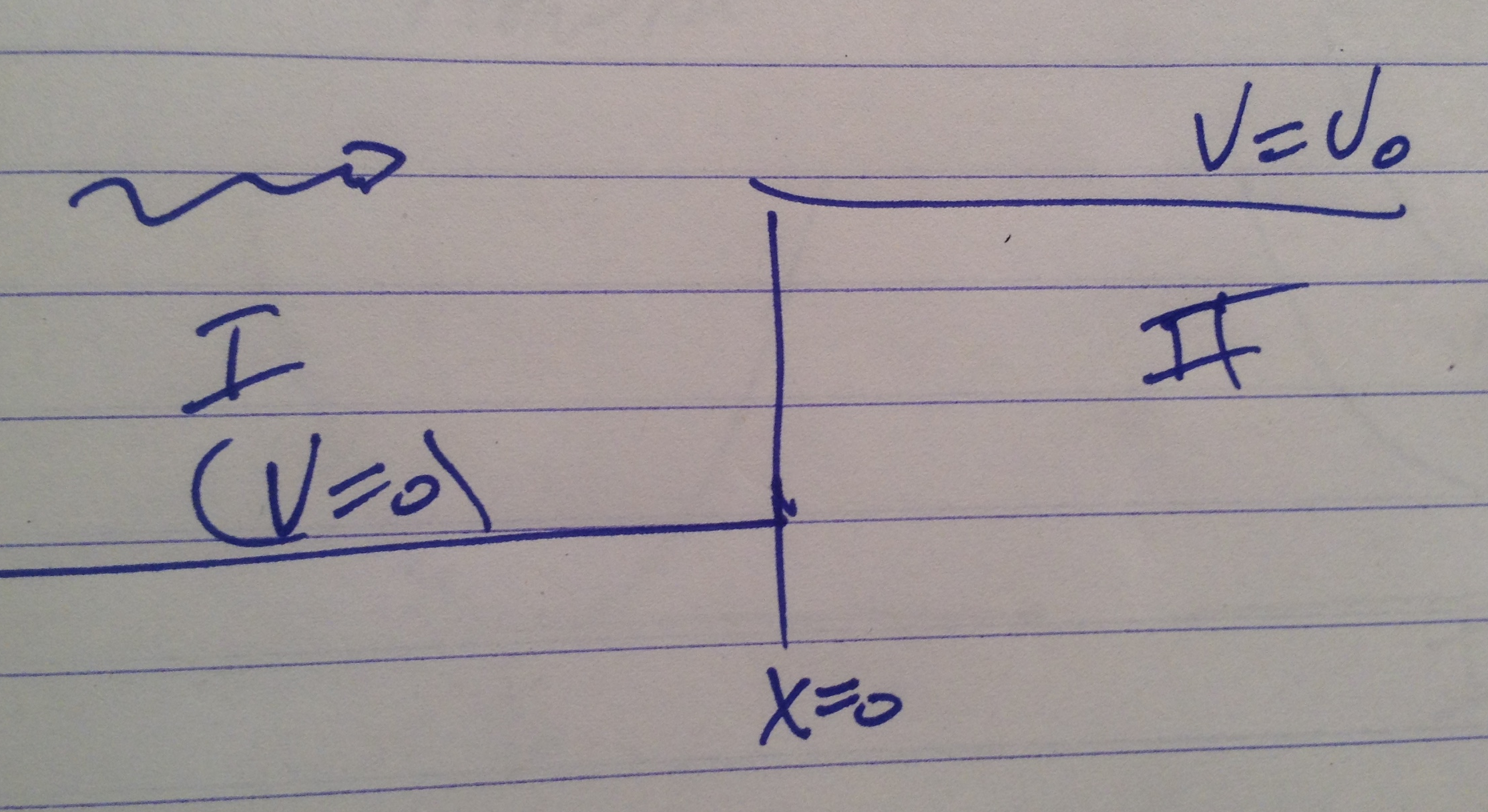
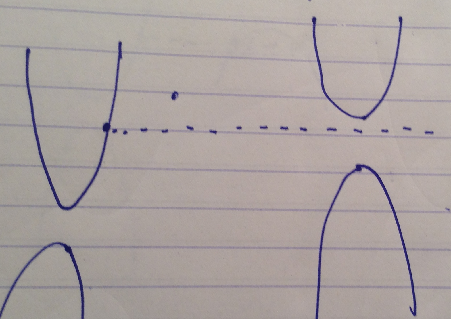
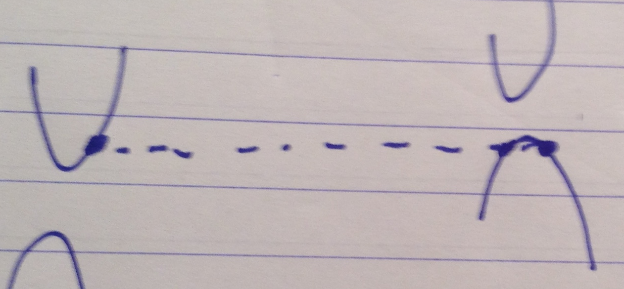
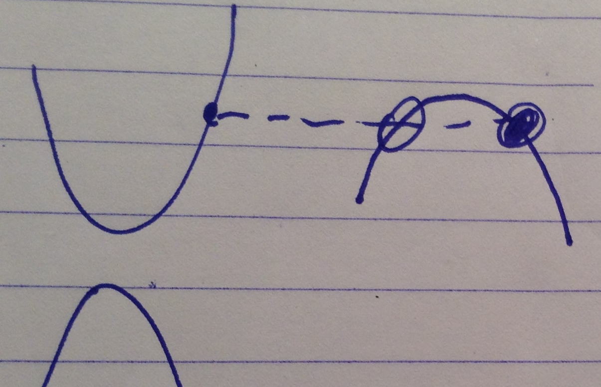
In one dimension, the parity operation is just inversion. In two dimensions, this is a set of flipping operations on two axes fig. 2.
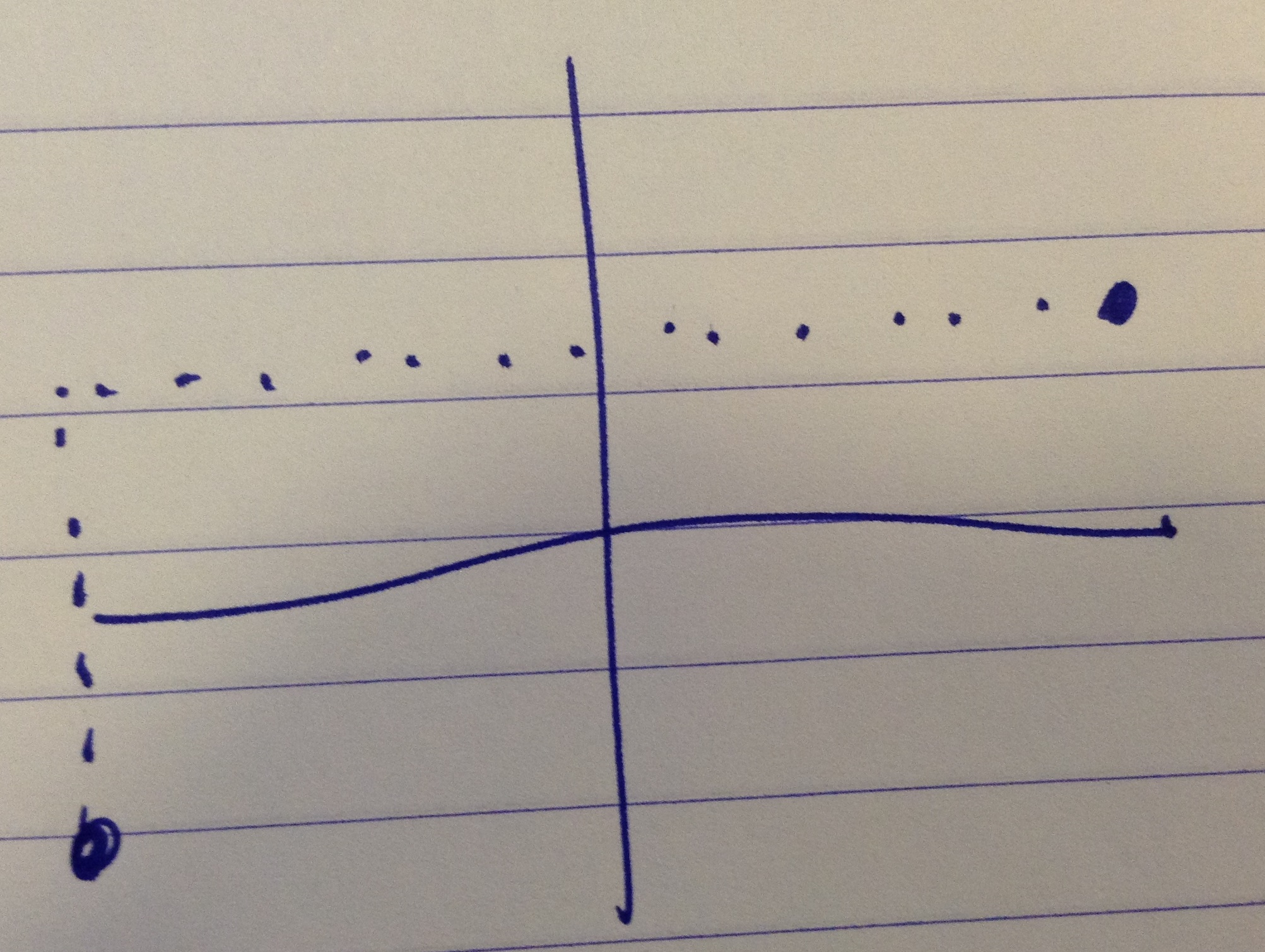
fig. 2. 2D parity operation
The operational effects of this operator are
\begin{equation}\label{eqn:qmLecture11:400}
\begin{aligned}
\hat{x} &\rightarrow – \hat{x} \\
\hat{p} &\rightarrow – \hat{p}.
\end{aligned}
\end{equation}
Acting again with the parity operator produces the original value, so it is its own inverse, and \( \hat{\Pi}^\dagger = \hat{\Pi} = \hat{\Pi}^{-1} \). In an expectation value
\begin{equation}\label{eqn:qmLecture11:420}
\bra{ \hat{\Pi} \psi } \hat{x} \ket{ \hat{\Pi} \psi } = – \bra{\psi} \hat{x} \ket{\psi}.
\end{equation}
This means that
\begin{equation}\label{eqn:qmLecture11:440}
\hat{\Pi}^\dagger \hat{x} \hat{\Pi} = – \hat{x},
\end{equation}
or
\begin{equation}\label{eqn:qmLecture11:460}
\hat{x} \hat{\Pi} = – \hat{\Pi} \hat{x},
\end{equation}
\begin{equation}\label{eqn:qmLecture11:480}
\begin{aligned}
\hat{x} \hat{\Pi} \ket{x_0}
&= – \hat{\Pi} \hat{x} \ket{x_0} \\
&= – \hat{\Pi} x_0 \ket{x_0} \\
&= – x_0 \hat{\Pi} \ket{x_0}
\end{aligned}
\end{equation}
so
\begin{equation}\label{eqn:qmLecture11:500}
\hat{\Pi} \ket{x_0} = \ket{-x_0}.
\end{equation}
Acting on a wave function
\begin{equation}\label{eqn:qmLecture11:520}
\begin{aligned}
\bra{x} \hat{\Pi} \ket{\psi}
&=
\braket{-x}{\psi} \\
&= \psi(-x).
\end{aligned}
\end{equation}
What does this mean for eigenfunctions. Eigenfunctions are supposed to form irreducible representations of the group. The group has just two elements
\begin{equation}\label{eqn:qmLecture11:540}
\setlr{ 1, \hat{\Pi} },
\end{equation}
where \( \hat{\Pi}^2 = 1 \).
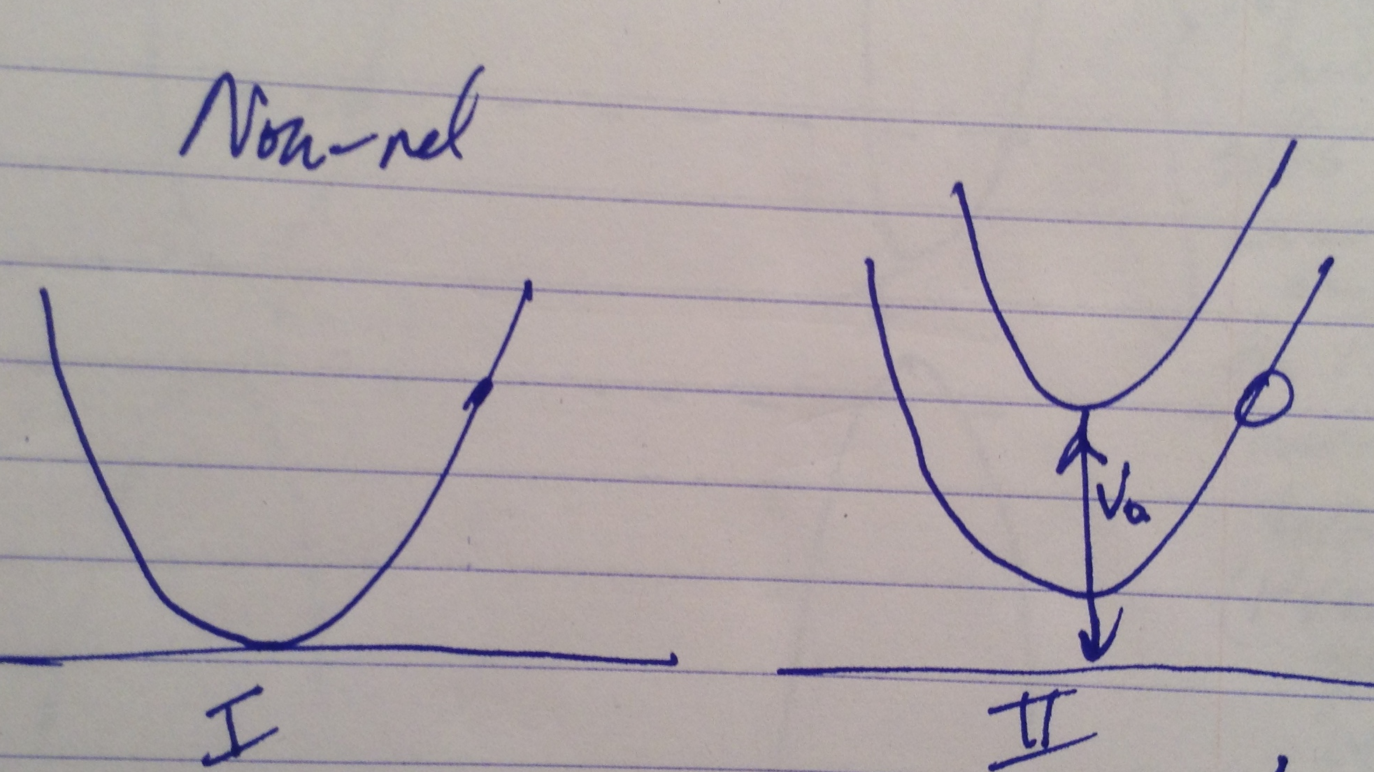
Suppose we have a Hamiltonian
\begin{equation}\label{eqn:qmLecture11:560}
H = \frac{\hat{p}^2}{2m} + V(\hat{x}),
\end{equation}
where \( V(\hat{x}) \) is even ( \( \antisymmetric{V(\hat{x})}{\hat{\Pi} } = 0 \) ). The squared momentum commutes with the parity operator
\begin{equation}\label{eqn:qmLecture11:580}
\begin{aligned}
\antisymmetric{\hat{p}^2}{\hat{\Pi}}
&=
\hat{p}^2 \hat{\Pi}
– \hat{\Pi} \hat{p}^2 \\
&=
\hat{p}^2 \hat{\Pi}
– (\hat{\Pi} \hat{p}) \hat{p} \\
&=
\hat{p}^2 \hat{\Pi}
-(- \hat{p} \hat{\Pi}) \hat{p} \\
&=
\hat{p}^2 \hat{\Pi}
+ \hat{p} (-\hat{p} \hat{\Pi}) \\
&=
0.
\end{aligned}
\end{equation}
Only two functions are possible in the symmetry set \( \setlr{ \Psi(x), \hat{\Pi} \Psi(x) } \), since
\begin{equation}\label{eqn:qmLecture11:600}
\begin{aligned}
\hat{\Pi}^2 \Psi(x)
&= \hat{\Pi} \Psi(-x) \\
&= \Psi(x).
\end{aligned}
\end{equation}
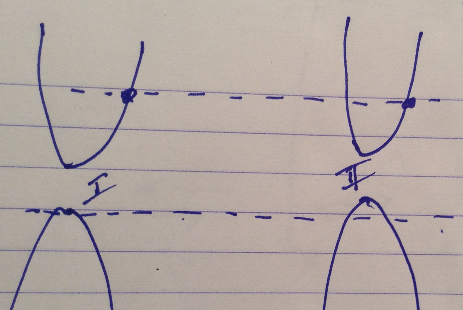
This symmetry severely restricts the possible solutions, making it so there can be only one dimensional forms of this problem with solutions that are either even or odd respectively
\begin{equation}\label{eqn:qmLecture11:620}
\begin{aligned}
\phi_e(x) &= \psi(x ) + \psi(-x) \\
\phi_o(x) &= \psi(x ) – \psi(-x).
\end{aligned}
\end{equation}
References
[1] Jun John Sakurai and Jim J Napolitano. Modern quantum mechanics. Pearson Higher Ed, 2014.