math and physics play

Simple Norton equivalents

November 10, 2014 ece1254 , ,

[Click here for a PDF of this post with nicer formatting]

The problem set contained a circuit with constant voltage source that made the associated Nodal matrix non-symmetric. There was a hint that this source \( V_s \) and its internal resistance \( R_s \) can likely be replaced by a constant current source.

Here two voltage source configurations will be compared to a current source configuration, with the assumption that equivalent circuit configurations can be found.

First voltage source configuration

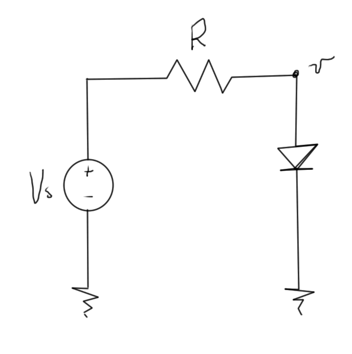
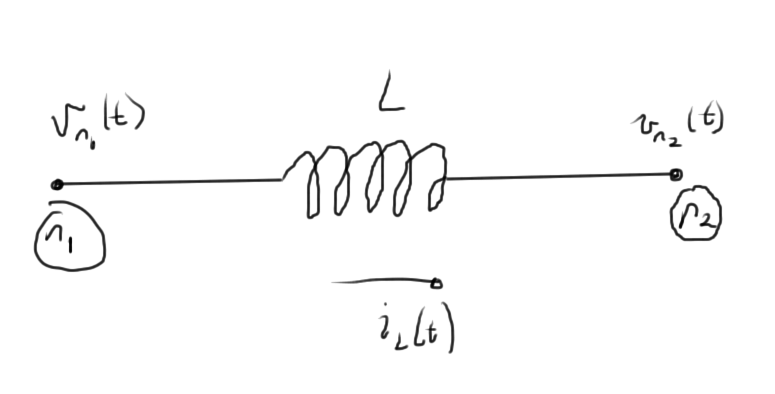
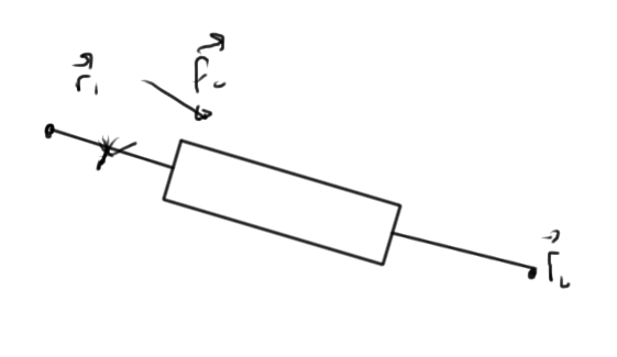
First consider the source and internal series resistance configuration sketched in fig. 1, with a purely resistive load.

nortonEquivalentFig1

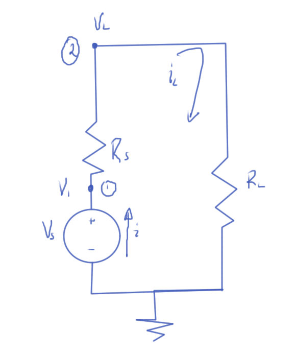
fig. 1. First voltage source configuration

The nodal equations for this system are

  1. \( -i_L + (V_1 – V_L) Z_s = 0 \)
  2. \( V_L Z_L + (V_L – V_1) Z_s = 0 \)
  3. \( V_1 = V_s \)

In matrix form these are

\begin{equation}\label{eqn:simpleNortonEquivalents:20}
\begin{bmatrix}
Z_s & -Z_s & -1 \\
-Z_s & Z_s + Z_L & 0 \\
1 & 0 & 0
\end{bmatrix}
\begin{bmatrix}
V_1 \\
V_L \\
i_L
\end{bmatrix}
=
\begin{bmatrix}
0 \\
0 \\
V_s
\end{bmatrix}
\end{equation}

This has solution

\begin{equation}\label{eqn:simpleNortonEquivalents:40}
V_L = V_s \frac{ R_L }{R_L + R_s}
\end{equation}
\begin{equation}\label{eqn:simpleNortonEquivalents:100}
i_L = \frac{V_s}{R_L + R_s}
\end{equation}
\begin{equation}\label{eqn:simpleNortonEquivalents:120}
V_1 = V_s.
\end{equation}

Second voltage source configuration

Now consider the same voltage source, but with the series resistance location flipped as sketched in fig. 2.

nortonEquivalentFig2

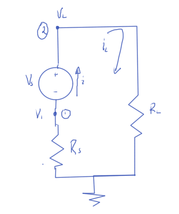
fig. 2. Second voltage source configuration

The nodal equations are

  1. \( V_1 Z_s + i_L = 0 \)
  2. \( -i_L + V_L Z_L = 0 \)
  3. \( V_L – V_1 = V_s \)

These have matrix form

\begin{equation}\label{eqn:simpleNortonEquivalents:60}
\begin{bmatrix}
Z_s & 0 & 1 \\
0 & Z_L & -1 \\
-1 & 1 & 0
\end{bmatrix}
\begin{bmatrix}
V_1 \\
V_L \\
i_L
\end{bmatrix}
=
\begin{bmatrix}
0 \\
0 \\
V_s
\end{bmatrix}
\end{equation}

This configuration has solution

\begin{equation}\label{eqn:simpleNortonEquivalents:50}
V_L = V_s \frac{ R_L }{R_L + R_s}
\end{equation}
\begin{equation}\label{eqn:simpleNortonEquivalents:180}
i_L = \frac{V_s}{R_L + R_s}
\end{equation}
\begin{equation}\label{eqn:simpleNortonEquivalents:200}
V_1 = -V_s \frac{ R_s }{R_L + R_s}
\end{equation}

Observe that the voltage at the load node and the current through this impedance is the same in both circuit configurations. The internal node voltage is different in each case, but that has no measurable effect on the external load.

Current configuration

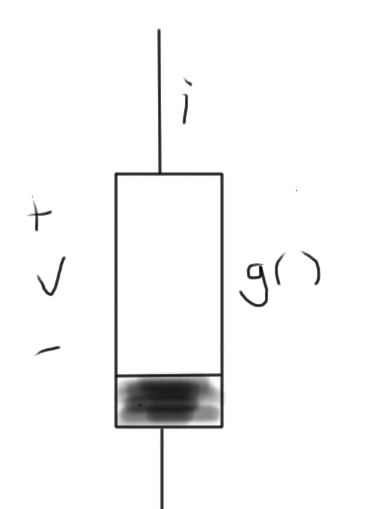
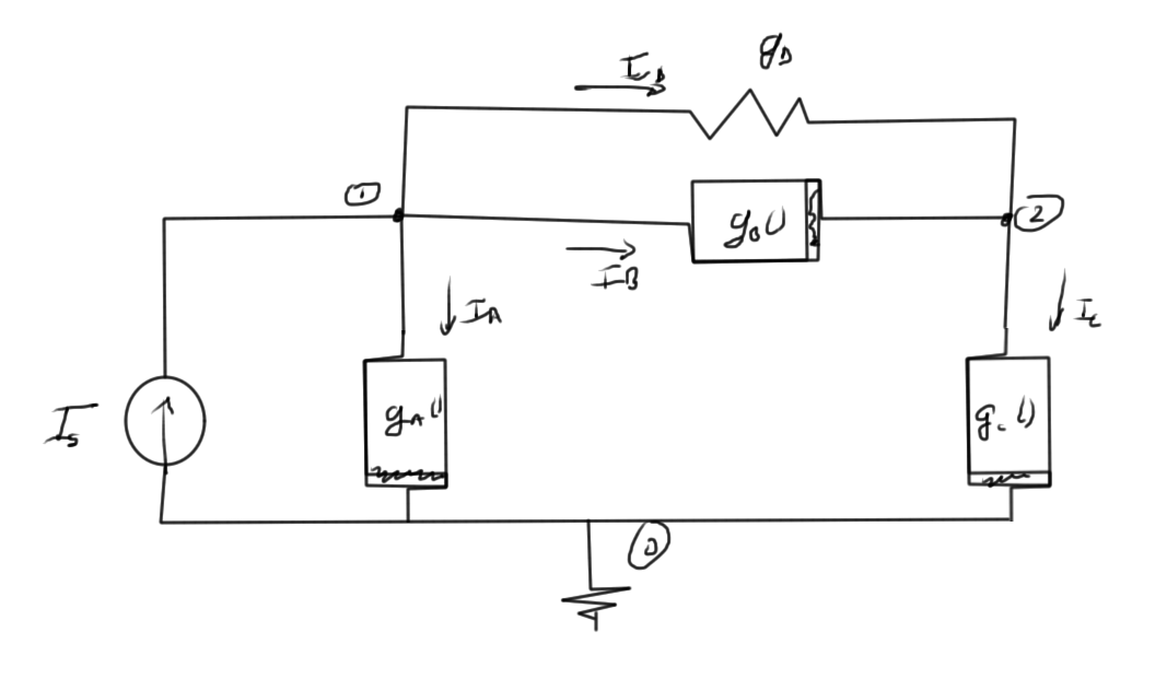
Now consider a current source and internal parallel resistance as sketched in fig. 3.

nortonEquivalentFig3

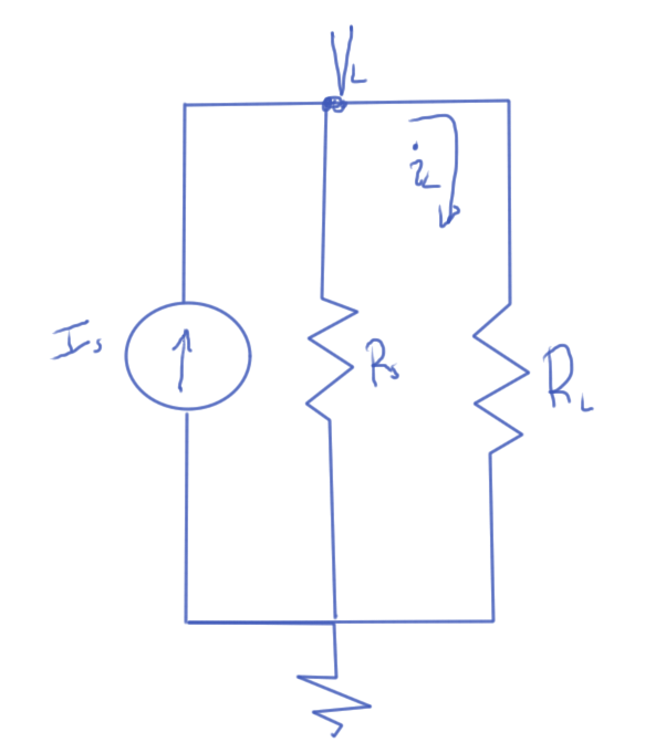
fig. 3. Current source configuration

There is only one nodal equation for this circuit

  1. \( -I_s + V_L Z_s + V_L Z_L = 0 \)

The load node voltage and current follows immediately

\begin{equation}\label{eqn:simpleNortonEquivalents:80}
V_L = \frac{I_s}{Z_L + Z_s}
\end{equation}
\begin{equation}\label{eqn:simpleNortonEquivalents:140}
i_L = V_L Z_L = \frac{Z_L I_s}{Z_L + Z_s}
\end{equation}

The goal is to find a value for \( I_L \) so that the voltage and currents at the load node match either of the first two voltage source configurations. It has been assumed that the desired parallel source resistance is the same as the series resistance in the voltage configurations. That was just a guess, but it ends up working out.

From \ref{eqn:simpleNortonEquivalents:80} and \ref{eqn:simpleNortonEquivalents:40} that equivalent current source can be found from

\begin{equation}\label{eqn:simpleNortonEquivalents:160}
V_L = V_s \frac{ R_L }{R_L + R_s} = \frac{I_s}{Z_L + Z_s},
\end{equation}

or

\begin{equation}\label{eqn:simpleNortonEquivalents:220}
I_s
=
V_s \frac{ R_L (Z_L + Z_s)}{R_L + R_s}
=
\frac{V_s}{R_S} \frac{ R_s R_L (Z_L + Z_s)}{R_L + R_s}
\end{equation}

\begin{equation}\label{eqn:simpleNortonEquivalents:240}
\boxed{
I_s
=
\frac{V_s}{R_S}.
}
\end{equation}

The load is expected to be the same through the load, and is

\begin{equation}\label{eqn:simpleNortonEquivalents:n}
i_L = V_L Z_L =
= V_s \frac{ R_L Z_L }{R_L + R_s}
= \frac{ V_s }{R_L + R_s},
\end{equation}

which matches \ref{eqn:simpleNortonEquivalents:100}.

Remarks

The equivalence of the series voltage source configurations with the parallel
current source configuration has been demonstrated with a resistive load. This
is a special case of the more general Norton’s theorem, as detailed in [2] and
[1] \S 5.1. Neither of those references prove the theorem. Norton’s theorem allows the equivalent current and resistance to be calculated without actually solving the system. Using that method, the parallel resistance equivalent follows by summing all the resistances in the source circuit with all the voltage sources shorted. Shorting the voltage sources in this source circuit results in the same configuration. It was seen directly in the two voltage source configurations that it did not matter, from the point of view of the external load, which sequence the internal series resistance and the voltage source were placed in did not matter. That becomes obvious with knowledge of Norton’s theorem, since shorting the voltage sources leaves just the single resistor in both cases.

References

[1] J.D. Irwin. Basic Engineering Circuit Analysis. Macillian, 1993.

[2] Wikipedia. Norton’s theorem — wikipedia, the free encyclopedia, 2014. URL https://en.wikipedia.org/w/index.php?title=Norton\%27s_theorem&oldid=629143825. [Online; accessed 1-November-2014].

ECE1254H Modeling of Multiphysics Systems. Lecture 13: Continuation parameters and Simulation of dynamical systems. Taught by Prof. Piero Triverio

October 29, 2014 ece1254 , ,

[Click here for a PDF of this post with nicer formatting]

Disclaimer

Peeter’s lecture notes from class. These may be incoherent and rough.

Singular Jacobians

(mostly on slides)

There is the possiblity of singular Jacobians to consider. FIXME: not sure how this system represented that. Look on slides.

lecture13Fig1

fig. 1. Diode system that results in singular Jacobian

\begin{equation}\label{eqn:multiphysicsL13:20}
\tilde{f}(v(\lambda), \lambda) = i(v) – \inv{R}( v – \lambda V_s ) = 0.
\end{equation}

An alternate continuation scheme uses

\begin{equation}\label{eqn:multiphysicsL13:40}
\tilde{F}(\Bx(\lambda), \lambda) = \lambda F(\Bx(\lambda)) + (1-\lambda) \Bx(\lambda).
\end{equation}

This scheme has

\begin{equation}\label{eqn:multiphysicsL13:60}
\tilde{F}(\Bx(0), 0) = 0
\end{equation}
\begin{equation}\label{eqn:multiphysicsL13:80}
\tilde{F}(\Bx(1), 1) = F(\Bx(1)),
\end{equation}

and for one variable, easy to compute Jacobian at the origin, or the original Jacobian at \( \lambda = 1 \)

\begin{equation}\label{eqn:multiphysicsL13:100}
\PD{x}{\tilde{F}}(x(0), 0) = I
\end{equation}
\begin{equation}\label{eqn:multiphysicsL13:120}
\PD{x}{\tilde{F}}(x(1), 1) = \PD{x}{F}(x(1))
\end{equation}

Simulation of dynamical systems

Example high level system in fig. 2.

lecture13Fig2

fig. 2. Complex time dependent system

Assembling equations automatically for dynamical systems

RC circuit

To demonstrate the method by example consider the RC circuit fig. 3 which has time dependence that must be considered

lecture13Fig3

fig. 3. RC circuit

The unknowns are \( v_1(t), v_2(t) \).

The equations (KCLs) at each of the nodes are

  1. \(
    \frac{v_1(t)}{R_1}
    + C_1 \frac{dv_1}{dt}
    + \frac{v_1(t) – v_2(t)}{R_2}
    + C_2 \frac{d(v_1 – v_2)}{dt}
    – i_{s,1}(t) = 0
    \)
  2. \(
    \frac{v_2(t) – v_1(t)}{R_2}
    + C_2 \frac{d(v_2 – v_1)}{dt}
    + \frac{v_2(t)}{R_3}
    + C_3 \frac{dv_2}{dt}
    – i_{s,2}(t)
    = 0
    \)

This has the matrix form
\begin{equation}\label{eqn:multiphysicsL13:140}
\begin{bmatrix}
Z_1 + Z_2 & – Z_2 \\
-Z_2 & Z_2 + Z_3
\end{bmatrix}
\begin{bmatrix}
v_1(t) \\
v_2(t)
\end{bmatrix}
+
\begin{bmatrix}
C_1 + C_2 & -C_2 \\
– C_2 & C_2 + C_3
\end{bmatrix}
\begin{bmatrix}
\frac{dv_1(t)}{dt} \\
\frac{dv_2(t}{dt})
\end{bmatrix}
=
\begin{bmatrix}
1 & 0 \\
0 & 1
\end{bmatrix}
\begin{bmatrix}
i_{s,1}(t) \\
i_{s,2}(t)
\end{bmatrix}.
\end{equation}

Observe that the capacitor between node 2 and 1 is associated with a stamp of the form

\begin{equation}\label{eqn:multiphysicsL13:180}
\begin{bmatrix}
C_2 & -C_2 \\
-C_2 & C_2
\end{bmatrix},
\end{equation}

very much like the impedance stamps of the resistor node elements.

The RC circuit problem has the abstract form

\begin{equation}\label{eqn:multiphysicsL13:160}
G \Bx(t) + C \frac{d\Bx(t)}{dt} = B \Bu(t),
\end{equation}

which is more general than a state space equation of the form

\begin{equation}\label{eqn:multiphysicsL13:200}
\frac{d\Bx(t)}{dt} = A \Bx(t) + B \Bu(t).
\end{equation}

Such a system may be represented diagramatically as in fig. 4.

lecture13Fig4

fig. 4. State space system

The \( C \) factor in this capacitance system, is generally not invertable. For example, if consider a 10 node system with only one capacitor, for which \( C \) will be mostly zeros.
In a state space system, in all equations we have a derivative. All equations are dynamical.

The time dependent MNA system for the RC circuit above, contains a mix of dynamical and algebraic equations. This could, for example, be a pair of equations like

\begin{equation}\label{eqn:multiphysicsL13:240}
\frac{dx_1}{dt} + x_2 + 3 = 0
\end{equation}
\begin{equation}\label{eqn:multiphysicsL13:260}
x_1 + x_2 + 3 = 0
\end{equation}

How to handle inductors

A pair of nodes that contains an inductor element, as in fig. 5, has to be handled specially.

lecture13Fig5

fig. 5. Inductor configuration

The KCL at node 1 has the form

\begin{equation}\label{eqn:multiphysicsL13:280}
\cdots + i_L(t) + \cdots = 0,
\end{equation}

where

\begin{equation}\label{eqn:multiphysicsL13:300}
v_{n_1}(t) – v_{n_2}(t) = L \frac{d i_L}{dt}.
\end{equation}

It is possible to express this in terms of \( i_L \), the variable of interest

\begin{equation}\label{eqn:multiphysicsL13:320}
i_L(t) = \inv{L} \int_0^t \lr{ v_{n_1}(\tau) – v_{n_2}(\tau) } d\tau
+ i_L(0).
\end{equation}

Expressing the problem directly in terms of such integrals makes the problem harder to solve, since the usual differential equation toolbox cannot be used directly. An integro-differential toolbox would have to be developed. What can be done instead is to introduce an additional unknown for each inductor current derivative \( di_L/dt \), for which an additional MNA row is introduced for that inductor scaled voltage difference.

Numerical solution of differential equations

Consider the one variable system

\begin{equation}\label{eqn:multiphysicsL13:340}
G x(t) + C \frac{dx}{dt} = B u(t),
\end{equation}

given an initial condition \( x(0) = x_0 \). Imagine that this system has the solution sketched in fig. 6.

lecture13Fig6

fig. 6. Discrete time sampling

Very roughly, the steps for solution are of the form

  1. Discretize time
  2. Aim to find the solution at \( t_1, t_2, t_3, \cdots \)
  3. Use a finite difference formula to approximate the derivative.

There are various schemes that can be used to discretize, and compute the finite differences.

Forward Euler method

\index{forward Euler method}

One such scheme is to use the forward differences, as in fig. 7, to approximate the derivative

\begin{equation}\label{eqn:multiphysicsL13:360}
\dot{x}(t_n) \approx \frac{x_{n+1} – x_n}{\Delta t}.
\end{equation}

lecture13Fig7

fig. 7. Forward difference derivative approximation

Introducing this into \ref{eqn:multiphysicsL13:340} gives

\begin{equation}\label{eqn:multiphysicsL13:350}
G x_n + C \frac{x_{n+1} – x_n}{\Delta t} = B u(t_n),
\end{equation}

or

\begin{equation}\label{eqn:multiphysicsL13:380}
C x_{n+1} = \Delta t B u(t_n) – \Delta t G x_n + C x_n.
\end{equation}

The coefficient \( C \) must be invertable, and the next point follows immediately

\begin{equation}\label{eqn:multiphysicsL13:381}
x_{n+1} = \frac{\Delta t B}{C} u(t_n)
+ x_n \lr{ 1 – \frac{\Delta t G}{C} }.
\end{equation}

Current collection of multiphysics modeling notes (ece1254)

October 27, 2014 ece1254

I’ve now posted
v.1 of my current notes collection for “Modeling of Multiphysics Systems” (ECE1254H1F), a course I’m now taking taught by Prof. Piero Triverio. This includes the following individual lecture or personal notes, which may or may not have been posted as separate blog entries:

October 27, 2014 Struts and Joints, Node branch formulation

October 24, 2014 Conjugate gradient method

October 22, 2014 Nonlinear equations

October 22, 2014 Conjugate gradient methods

October 21, 2014 Nonlinear systems

October 21, 2014 Sparse factorization and iterative methods

October 15, 2014 Illustrating the LU algorthm with pivots by example

October 14, 2014 Modified Nodal Analysis

October 09, 2014 Numerical LU example where pivoting is required

October 09, 2014 Numeric LU factorization example

October 02, 2014 Singular Value Decomposition

October 01, 2014 Matrix norm, singular decomposition, and conditioning number

September 30, 2014 Numerical error and conditioning.

September 26, 2014 Solving large systems

September 24, 2014 Nodal Analysis

September 23, 2014 Assembling system equations automatically

September 23, 2014 Analogies to circuit systems

ECE1254H Modeling of Multiphysics Systems. Lecture 12: Struts and Joints, Node branch formulation. Taught by Prof. Piero Triverio

October 27, 2014 ece1254 , , , ,

[Click here for a PDF of this post with nicer formatting]

Disclaimer

Peeter’s lecture notes from class. These may be incoherent and rough.

Struts and Joints, Node branch formulation

Let’s consider the simple strut system of fig. 1 again.

lecture12Fig1

fig. 1. Simple strut system


Our unknowns are

  1. Forces at each of the points we have a force with two components
    \begin{equation}\label{eqn:multiphysicsL12:20}
    \Bf_A = \lr{ f_{A,x}, f_{A,y} }
    \end{equation}We construct a total force vector\begin{equation}\label{eqn:multiphysicsL12:40}
    \Bf =
    \begin{bmatrix}
    f_{A,x} \\
    f_{A,y} \\
    f_{B,x} \\
    f_{B,y} \\
    \vdots
    \end{bmatrix}
    \end{equation}
  2. Positions of the joints\begin{equation}\label{eqn:multiphysicsL12:60}
    \Br =
    \begin{bmatrix}
    x_1 \\
    y_1 \\
    y_1 \\
    y_2 \\
    \vdots
    \end{bmatrix}
    \end{equation}

Our given variables are

  1. The load force \( \Bf_L \).
  2. The joint positions at rest.
  3. parameter of struts.

Conservation laws

The conservation laws are

\begin{equation}\label{eqn:multiphysicsL12:80}
\Bf_A + \Bf_B + \Bf_C = 0
\end{equation}
\begin{equation}\label{eqn:multiphysicsL12:100}
-\Bf_C + \Bf_D + \Bf_L = 0
\end{equation}

which we can put in matrix form

\begin{equation}\label{eqn:multiphysicsL12:120}
\begin{bmatrix}
1 & 0 & 1 & 0 & 1 & 0 & 0 & 0 \\
0 & 1 & 0 & 1 & 0 & 0 & 0 & 0 \\
0 & 0 & 0 & 0 & -1 & 0 & 1 & 0 \\
0 & 1 & 0 & 1 & 0 & -1 & 0 & 1 \\
\end{bmatrix}
\begin{bmatrix}
f_{A,x} \\
f_{A,y} \\
f_{B,x} \\
f_{B,y} \\
f_{C,x} \\
f_{C,y} \\
f_{D,x} \\
f_{D,y}
\end{bmatrix}
=
\begin{bmatrix}
0 \\
0 \\
-f_{L,x} \\
-f_{L,y}
\end{bmatrix}
\end{equation}

Here the block matrix is called the incidence matrix \( \BA \), and we write

\begin{equation}\label{eqn:multiphysicsL12:160}
A \Bf = \Bf_L.
\end{equation}

Constitutive laws

Given a pair of nodes as in fig. 2.

lecture12Fig2

fig. 2. Strut spanning nodes


each component has an equation relating the reaction forces of that strut based on the positions

\begin{equation}\label{eqn:multiphysicsL12:180}
f_{c,x} = S_x \lr{ x_1 – x_2, y_1 – y_2, p_c }
\end{equation}
\begin{equation}\label{eqn:multiphysicsL12:200}
f_{c,y} = S_y \lr{ x_1 – x_2, y_1 – y_2, p_c },
\end{equation}

where \( p_c \) represent the parameters of the system. We write

\begin{equation}\label{eqn:multiphysicsL12:220}
\Bf =
\begin{bmatrix}
f_{A,x} \\
f_{A,y} \\
f_{B,x} \\
f_{B,y} \\
\vdots
\end{bmatrix}
=
\begin{bmatrix}
S_x \lr{ x_1 – x_2, y_1 – y_2, p_c } \\
S_y \lr{ x_1 – x_2, y_1 – y_2, p_c } \\
\vdots
\end{bmatrix},
\end{equation}

or

\begin{equation}\label{eqn:multiphysicsL12:260}
\Bf = S(\Br)
\end{equation}

Putting the pieces together

The node branch formulation is

\begin{equation}\label{eqn:multiphysicsL12:280}
\begin{aligned}
A \Bf – \Bf_L &= 0 \\
\Bf – S(\Br) &= 0
\end{aligned}
\end{equation}

We’ll want to approximate this system using the Jacobian methods discussed, and can expect the cost of that Jacobian calculation to potentially be expensive. To move to the nodal formulation we eliminate forces (the equivalent of currents in this system)

\begin{equation}\label{eqn:multiphysicsL12:320}
A S(\Br) – \Bf_L = 0
\end{equation}

We cannot use this nodal formulation when we have struts that are so stiff that the positions of some of the nodes are fixed, but can work around that as before by introducing an additional unknown for each component of such a strut.

Damped Newton’s method

We want to be able to deal with the oscillation that we can have in examples like that of fig. 3.

lecture12Fig3

fig. 3. Oscillatory Newton’s iteration


Large steps can be dangerous. We want to modify Newton’s method as follows

Our algorithm is

  • Guess \( \Bx^0, k = 0 \).
  • REPEAT
  • Compute \( F \) and \( J_F \) at \( \Bx^k \)
  • Solve linear system \( J_F(\Bx^k) \Delta \Bx^k = – F(\Bx^k) \)
  • \( \Bx^{k+1} = \Bx^k + \alpha^k \Delta \Bx^k \)
  • \( k = k + 1 \)
  • UNTIL converged

with \( \alpha^k = 1 \) we have standard Newton’s method. We want to pick \( \alpha^k \) so that we minimize

Continuation parameters

Newton’s method converges given a close initial guess. We can generate a sequence of problems where the previous problem generates a good initial guess for the next problem.

An example is a heat conducting bar, with a final heat distribution. We can start the numeric iteration with \( T = 0 \), and gradually increase the temperatures until we achieve the final desired heat distribution.

Suppose that we want to solve

\begin{equation}\label{eqn:multiphysicsL12:340}
F(\Bx) = 0.
\end{equation}

We modify this problem by introducing

\begin{equation}\label{eqn:multiphysicsL12:360}
\tilde{F}(\Bx(\lambda), \lambda) = 0,
\end{equation}

where

  • \( \tilde{F}(\Bx(0), 0) = 0 \) is easy to solve
  • \( \tilde{F}(\Bx(1), 1) = 0 \) is equivalent to \( F(\Bx) = 0 \).
  • (more on slides)

The source load stepping algorithm is

  • Solve \(\tilde{F}(\Bx(0), 0) = 0 \), with \( \Bx(\lambda_{\text{prev}} = \Bx(0) \)
  • (more on slides)

This can still have problems, for example, when the parameterization is multivalued as in fig. 4.

lecture12Fig4

fig. 4. Multivalued parameterization


We can attempt to adjust \( \lambda \) so that we move along the parameterization curve.

ECE1254H Modeling of Multiphysics Systems. Lecture 11: Nonlinear equations. Taught by Prof. Piero Triverio

October 22, 2014 ece1254 , , ,

[Click here for a PDF of this post with nicer formatting]

ECE1254H Modeling of Multiphysics Systems. Lecture 11: Nonlinear equations. Taught by Prof. Piero Triverio

Disclaimer

Peeter’s lecture notes from class. These may be incoherent and rough.

Solution of N nonlinear equations in N unknowns

We’d now like to move from solutions of nonlinear functions in one variable:

\begin{equation}\label{eqn:multiphysicsL11:200}
f(x^\conj) = 0,
\end{equation}

to multivariable systems of the form

\begin{equation}\label{eqn:multiphysicsL11:20}
\begin{aligned}
f_1(x_1, x_2, \cdots, x_N) &= 0 \\
\vdots & \\
f_N(x_1, x_2, \cdots, x_N) &= 0 \\
\end{aligned},
\end{equation}

where our unknowns are
\begin{equation}\label{eqn:multiphysicsL11:40}
\Bx =
\begin{bmatrix}
x_1 \\
x_2 \\
\vdots \\
x_N \\
\end{bmatrix}.
\end{equation}

Form the vector \( F \)

\begin{equation}\label{eqn:multiphysicsL11:60}
F(\Bx) =
\begin{bmatrix}
f_1(x_1, x_2, \cdots, x_N) \\
\vdots \\
f_N(x_1, x_2, \cdots, x_N) \\
\end{bmatrix},
\end{equation}

so that the equation to solve is

\begin{equation}\label{eqn:multiphysicsL11:80}
\boxed{
F(\Bx) = 0.
}
\end{equation}

The Taylor expansion of \( F \)

around point \( \Bx_0 \) is

\begin{equation}\label{eqn:multiphysicsL11:100}
F(\Bx) = F(\Bx_0) +
\underbrace{ J_F(\Bx_0) }_{Jacobian}
\lr{ \Bx – \Bx_0},
\end{equation}

where the Jacobian is

\begin{equation}\label{eqn:multiphysicsL11:120}
J_F(\Bx_0)
=
\begin{bmatrix}
\PD{x_1}{f_1} & \cdots & \PD{x_N}{f_1} \\
& \ddots & \\
\PD{x_1}{f_N} & \cdots & \PD{x_N}{f_N}
\end{bmatrix}
\end{equation}

Multivariable Newton’s iteration

Given \( \Bx^k \), expand \( F(\Bx) \) around \( \Bx^k \)

\begin{equation}\label{eqn:multiphysicsL11:140}
F(\Bx) \approx F(\Bx^k) + J_F(\Bx^k) \lr{ \Bx – \Bx^k }
\end{equation}

With the approximation

\begin{equation}\label{eqn:multiphysicsL11:160}
0 = F(\Bx^k) + J_F(\Bx^k) \lr{ \Bx^{k + 1} – \Bx^k },
\end{equation}

then multiplying by the inverse Jacobian, and rearranging, we have

\begin{equation}\label{eqn:multiphysicsL11:220}
\boxed{
\Bx^{k+1} = \Bx^k – J_F^{-1}(\Bx^k) F(\Bx^k).
}
\end{equation}

Our algorithm is

  • Guess \( \Bx^0, k = 0 \).
  • REPEAT
  • Compute \( F \) and \( J_F \) at \( \Bx^k \)
  • Solve linear system \( J_F(\Bx^k) \Delta \Bx^k = – F(\Bx^k) \)
  • \( \Bx^{k+1} = \Bx^k + \Delta \Bx^k \)
  • \( k = k + 1 \)
  • UNTIL converged

As with one variable, our convergence is after we have all of the convergence conditions satisfied

\begin{equation}\label{eqn:multiphysicsL11:240}
\begin{aligned}
\Norm{ \Delta \Bx^k } &< \epsilon_1 \\
\Norm{ F(\Bx^{k+1}) } &< \epsilon_2 \\
\frac{\Norm{ \Delta \Bx^k }}{\Norm{\Bx^{k+1}}} &< \epsilon_3 \\
\end{aligned}
\end{equation}

Typical termination is some multiple of eps, where eps is the machine precision. This may be something like:

\begin{equation}\label{eqn:multiphysicsL11:260}
4 \times N \times \text{eps},
\end{equation}

where \( N \) is the “size of the problem”. Sometimes we may be able to find meaningful values for the problem. For example, for a voltage problem, we may not be interested in precisions greater than a millivolt.

Automatic assembly of equations for nolinear system

Nonlinear circuits

We will start off considering a non-linear resistor, designated within a circuit as sketched in fig. 2.

lecture11Fig2

fig. 2. Non-linear resistor


Example: diode, with \( i = g(v) \), such as

\begin{equation}\label{eqn:multiphysicsL11:280}
i = I_0 \lr{ e^{v/{\eta V_T}} – 1 }.
\end{equation}

Consider the example circuit of fig. 3. KCL’s at each of the nodes are

lecture11Fig3

fig. 3. Example circuit


  1. \( I_A + I_B + I_D – I_s = 0 \)
  2. \( – I_B + I_C – I_D = 0 \)

Introducing the consistuative equations this is

  1. \( g_A(V_1) + g_B(V_1 – V_2) + g_D (V_1 – V_2) – I_s = 0 \)
  2. \( – g_B(V_1 – V_2) + g_C(V_2) – g_D (V_1 – V_2) = 0 \)

In matrix form this is
\begin{equation}\label{eqn:multiphysicsL11:300}
\begin{bmatrix}
g_D & -g_D \\
-g_D & g_D
\end{bmatrix}
\begin{bmatrix}
V_1 \\
V_2
\end{bmatrix}
+
\begin{bmatrix}
g_A(V_1) &+ g_B(V_1 – V_2) & & – I_s \\
&- g_B(V_1 – V_2) & + g_C(V_2) & \\
\end{bmatrix}
=
0
.
\end{equation}

We can write the entire system as

\begin{equation}\label{eqn:multiphysicsL11:320}
\boxed{
F(\Bx) = G \Bx + F'(\Bx) = 0.
}
\end{equation}

The first term, a product of a nodal matrix \( G \) represents the linear subnetwork, and is filled with the stamps we are already familiar with.

The second term encodes the relationships of the nonlinear subnetwork. This non-linear component has been marked with a prime to distinguish it from the complete network function that includes both linear and non-linear elements.

Observe the similarity with the stamp analysis that we did previously. With \( g_A() \) connected on one end to ground we have it only once in the resulting vector, whereas the nonlinear elements connected to two non-zero nodes in the network occur once with each sign.

Stamp for nonlinear resistor

For the non-linear circuit element of fig. 4.

lecture11Fig4

fig. 4. Non-linear resistor circuit element

The stamp is

fprimex

Stamp for Jacobian

\begin{equation}\label{eqn:multiphysicsL11:360}
J_F(\Bx^k) = G + J_{F’}(\Bx^k).
\end{equation}

Here the stamp for the Jacobian, an \( N \times N \) matrix, is

jacobianNonlinearPart