plane wave

Plane wave solution directly from Maxwell’s equations

May 6, 2015 math and physics play , , , ,

[Click here for a PDF of this post with nicer formatting]

Here’s a problem that I thought was fun, an exercise for the reader to show that the plane wave solution to Maxwell’s equations can be found with ease directly from Maxwell’s equations. This is in contrast to the what seems like the usual method of first showing that Maxwell’s equations imply wave equations for the fields, and then solving those wave equations.

Problem. \( \xcap \) oriented plane wave electric field ([1] ex. 4.1)

A uniform plane wave having only an \( x \) component of the electric field is traveling in the \( + z \) direction in an unbounded lossless, source-0free region. Using Maxwell’s equations write expressions for the electric and corresponding magnetic field intensities.

Answer

The phasor form of Maxwell’s equations for a source free region are

\begin{equation}\label{eqn:ExPlaneWave:40}
\spacegrad \cross \BE = -j \omega \BB
\end{equation}
\begin{equation}\label{eqn:ExPlaneWave:60}
\spacegrad \cross \BH = j \omega \BD
\end{equation}
\begin{equation}\label{eqn:ExPlaneWave:80}
\spacegrad \cdot \BD = 0
\end{equation}
\begin{equation}\label{eqn:ExPlaneWave:100}
\spacegrad \cdot \BB = 0.
\end{equation}

Since \( \BE = \xcap E(z) \), the magnetic field follows from \ref{eqn:ExPlaneWave:40}

\begin{equation}\label{eqn:ExPlaneWave:120}
-j \omega \BB
= \spacegrad \cross \BE
=
\begin{vmatrix}
\xcap & \ycap & \zcap \\
\partial_x & \partial_y & \partial_z \\
E & 0 & 0
\end{vmatrix}
=
\ycap \partial_z E(z)
– \zcap \partial_y E(z),
\end{equation}

or

\begin{equation}\label{eqn:ExPlaneWave:140}
\BB =
-\inv{j \omega} \partial_z E.
\end{equation}

This is constrained by \ref{eqn:ExPlaneWave:60}

\begin{equation}\label{eqn:ExPlaneWave:160}
j \omega \epsilon \xcap E
=
\inv{\mu} \spacegrad \cross \BB
=
-\inv{\mu j \omega}
\begin{vmatrix}
\xcap & \ycap & \zcap \\
\partial_x & \partial_y & \partial_z \\
0 & \partial_z E & 0
\end{vmatrix}
=
-\inv{\mu j \omega}
\lr{
-\xcap \partial_{z z} E
+ \zcap \partial_x \partial_z E
}
\end{equation}

Since \( \partial_x \partial_z E = \partial_z \lr{ \partial_x E } = \partial_z \inv{\epsilon} \spacegrad \cdot \BD = \partial_z 0 \), this means

\begin{equation}\label{eqn:ExPlaneWave:180}
\partial_{zz} E = -\omega^2 \epsilon\mu E = -k^2 E.
\end{equation}

This is the usual starting place that we use to show that the plane wave has an exponential form

\begin{equation}\label{eqn:ExPlaneWave:200}
\BE(z) =
\xcap
\lr{
E_{+} e^{-j k z}
+
E_{-} e^{j k z}
}.
\end{equation}

The magnetic field from \ref{eqn:ExPlaneWave:140} is

\begin{equation}\label{eqn:ExPlaneWave:220}
\BB
= \frac{j}{\omega} \lr{ -j k E_{+} e^{-j k z} + j k E_{-} e^{j k z} }
= \inv{c} \lr{ E_{+} e^{-j k z} – E_{-} e^{j k z} },
\end{equation}

or

\begin{equation}\label{eqn:ExPlaneWave:240}
\BH
= \inv{\mu c} \lr{ E_{+} e^{-j k z} – E_{-} e^{j k z} }
= \inv{\eta} \lr{ E_{+} e^{-j k z} – E_{-} e^{j k z} }.
\end{equation}

A solution requires zero divergence for the magnetic field, but that can be seen to be the case by inspection.

References

[1] Constantine A Balanis. Advanced engineering electromagnetics. Wiley New York, 1989.

Updated notes for ece1229 antenna theory

March 16, 2015 ece1229 , , , , , , , , , , , , , , , , , , , , , , , , , , , , , , , , , , , , , , , , , , , , , , , , , , , , , , , , , , , , , , , , , , , , , , , , , , , , , , , , , , , , , , , , , , , , , , , , , , , , , , , , , , , , , , , , , , , , , , , , , , , , , , , , , , , , , , , , , , , , , , , , , , , , ,

I’ve now posted a first update of my notes for the antenna theory course that I am taking this term at UofT.

Unlike most of the other classes I have taken, I am not attempting to take comprehensive notes for this class. The class is taught on slides which go by faster than I can easily take notes for (and some of which match the textbook closely). In class I have annotated my copy of textbook with little details instead. This set of notes contains musings of details that were unclear, or in some cases, details that were provided in class, but are not in the text (and too long to pencil into my book), as well as some notes Geometric Algebra formalism for Maxwell’s equations with magnetic sources (something I’ve encountered for the first time in any real detail in this class).

The notes compilation linked above includes all of the following separate notes, some of which have been posted separately on this blog:

Notes for Balantis chapter 4: linear wire antennas.

February 16, 2015 ece1229 , , , , , , , , , , , , , ,

[Click here for a PDF of this post with nicer formatting]

These are notes for the UofT course ECE1229, Advanced Antenna Theory, taught by Prof. Eleftheriades, covering ch. 4 [1] content.

Unlike most of the other classes I have taken, I am not attempting to take comprehensive notes for this class. The class is taught on slides that match the textbook so closely, there is little value to me taking notes that just replicate the text. Instead, I am annotating my copy of textbook with little details instead. My usual notes collection for the class will contain musings of details that were unclear, or in some cases, details that were provided in class, but are not in the text (and too long to pencil into my book.)

Magnetic Vector Potential.

In class and in the problem set \( \BA \) was referred to as the Magnetic Vector Potential.  I only recalled this referred to as the Vector Potential.  Prefixing this with magnetic seemed counter intuitive to me since it is generated by electric sources (charges and currents).
This terminology can be justified due to the fact that \( \BA \) generates the magnetic field by its curl. Some mention of this can be found in [4], which also points out that the Electric Potential refers to the scalar \( \phi \). Prof. Eleftheriades points out that Electric Vector Potential refers to the vector potential \( \BF \) generated by magnetic sources (because in that case the electric field is generated by the curl of \( \BF \).)

Plots of infinitesimal dipole radial dependence.

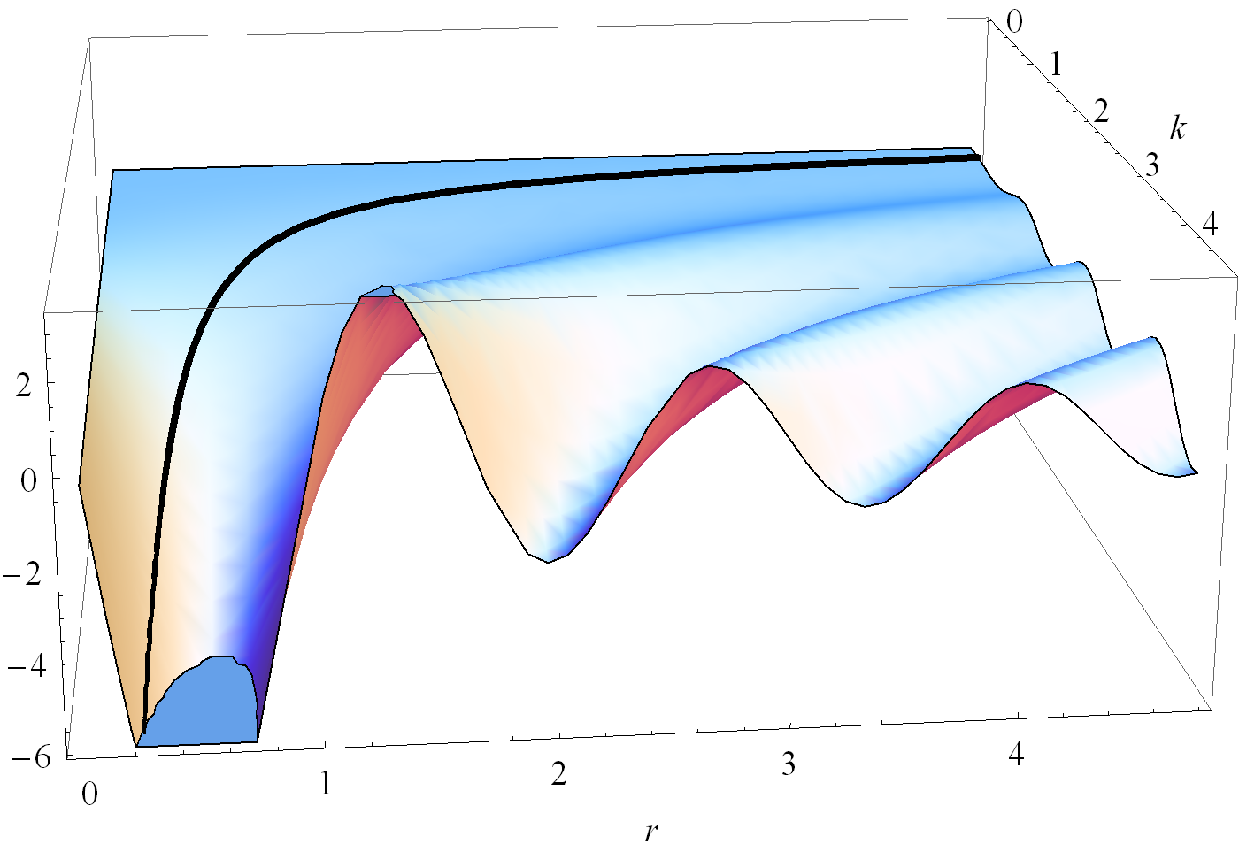
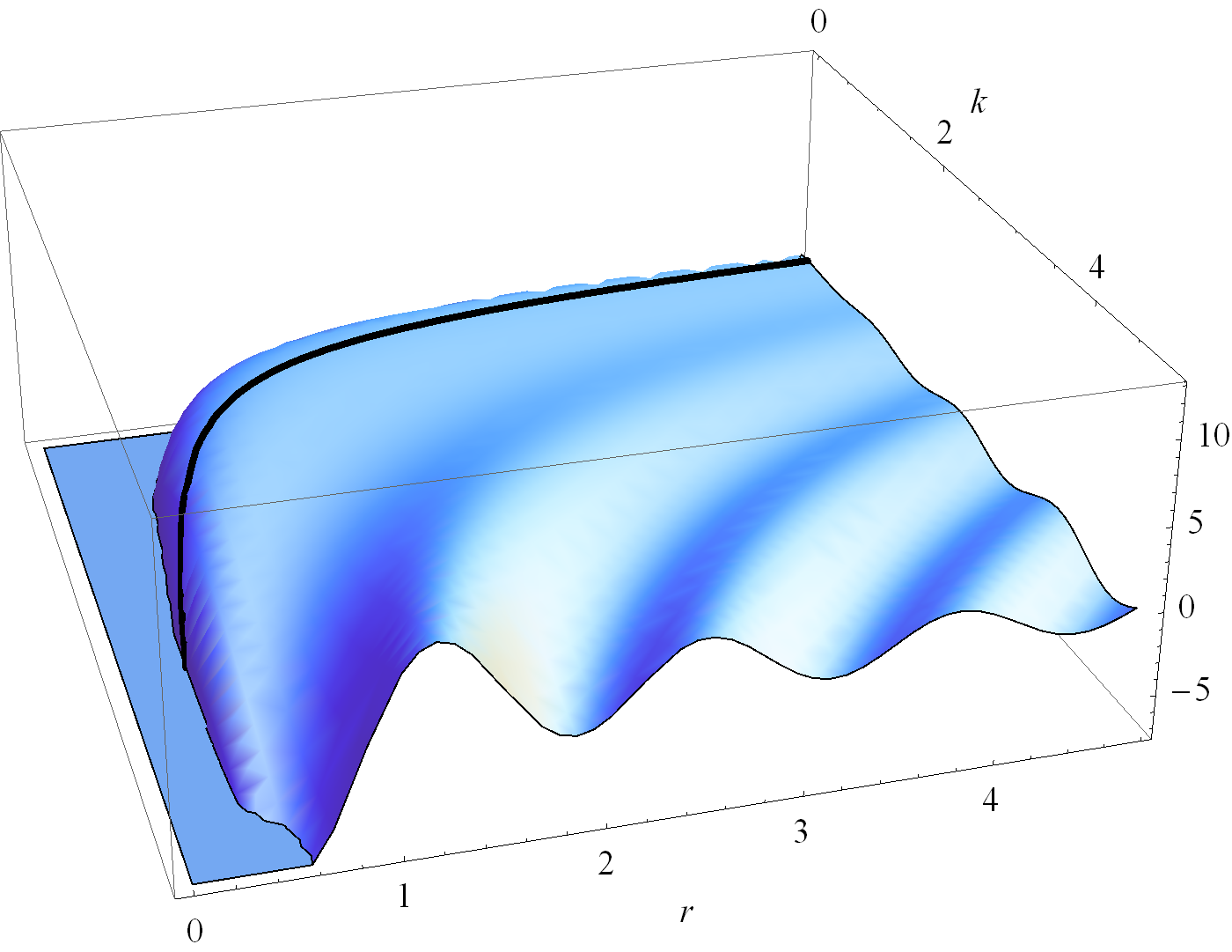
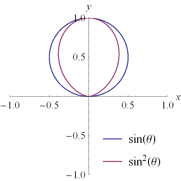
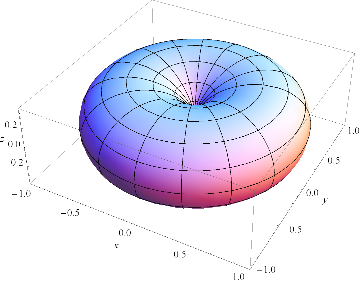
In section 4.2 of [1] are some discussions of the \( kr < 1 \), \( kr = 1 \), and \( kr > 1 \) radial dependence of the fields and power of a solution to an infinitesimal dipole system. Here are some plots of those \( k r \) dependence, along with the \( k r = 1 \) contour as a reference. All the \( \theta \) dependence and any scaling is left out.

The CDF notebook visualizeDipoleFields.cdf is available to interactively plot these, rotate the plots and change the ranges of what is plotted.

A plot of the real and imaginary parts of \( H_\phi = \frac{j k}{r} e^{-j k r} \lr{ 1-\frac{j}{k r} } \) can be found in fig. 1 and fig. 2.

infinitesimalDipoleHphiRealFig3pn

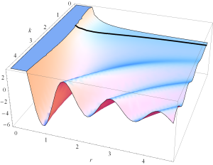
fig 1. Radial dependence of Re H_phi

infinitesimalDipoleHphiImagFig4pn

fig 2. Radial dependence of Im H_phi


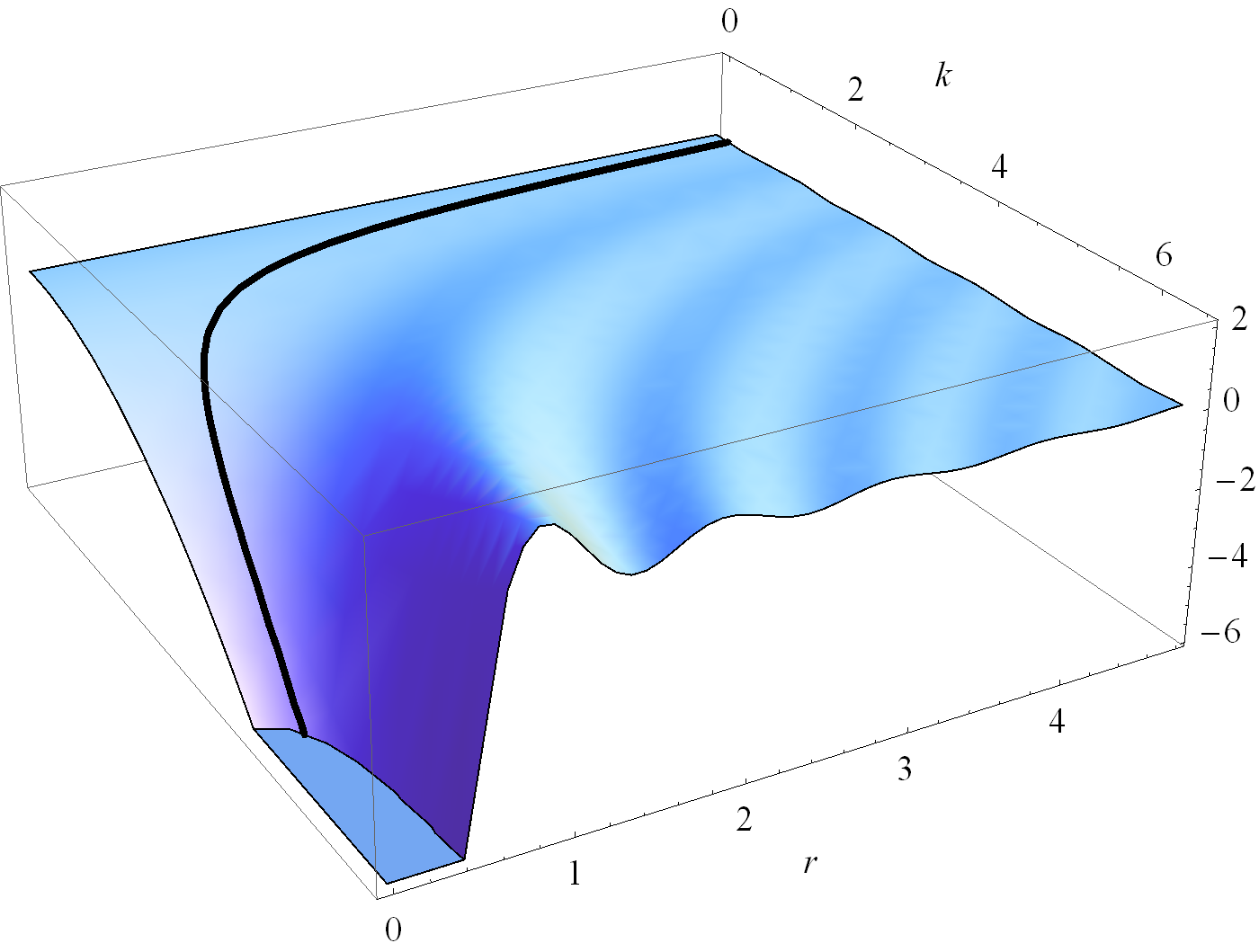
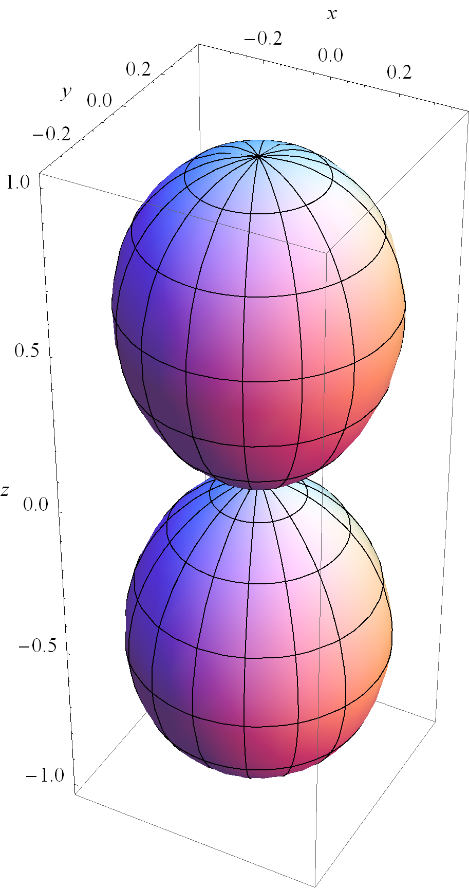
A plot of the real and imaginary parts of \( E_r = \inv{r^2} \lr{1-\frac{j}{k r}} e^{-j k r} \) can be found in fig. 3 and fig. 4.

infinitesimalDipoleErRealFig1pn

fig 3. Radial dependence of Re E_r

infinitesimalDipoleErImagFig2pn

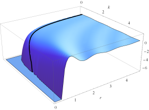
fig 4. Radial dependence of Im E_r


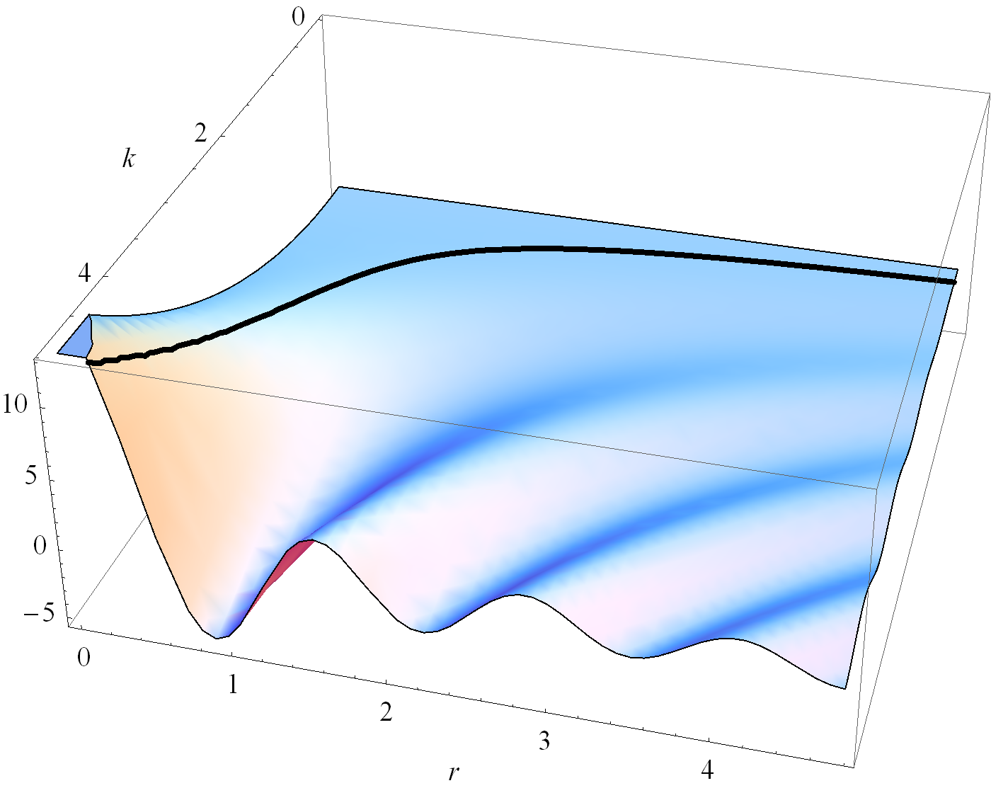
Finally, a plot of the real and imaginary parts of \( E_\theta = \frac{ j k }{r} \lr{1 -\frac{j}{k r} -\frac{1}{k^2 r^2} } e^{-j k r} \) can be found in fig. 5 and fig. 6.

infinitesimalDipoleEthetaRealFig5pn

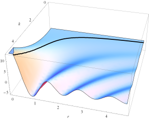
fig. 5. Radial dependence of Re E_theta

infinitesimalDipoleEthetaImagFig6pn

fig. 6. Radial dependence of Im E_theta


Electric Far field for a spherical potential.

It is interesting to look at the far electric field associated with an arbitrary spherical magnetic vector potential, assuming all of the radial dependence is in the spherical envelope. That is

\begin{equation}\label{eqn:chapter4Notes:20}
\BA = \frac{e^{-j k r}}{r} \lr{
\rcap a_r\lr{ \theta, \phi }
+\thetacap a_\theta\lr{ \theta, \phi }
+\phicap a_\phi\lr{ \theta, \phi }
}.
\end{equation}

The electric field is

\begin{equation}\label{eqn:chapter4Notes:40}
\BE = – j \omega \BA – j \frac{1}{\omega \mu_0 \epsilon_0 } \spacegrad \lr{\spacegrad \cdot \BA }.
\end{equation}

The divergence and gradient in spherical coordinates are

\begin{equation}\label{eqn:chapter4Notes:80}
\begin{aligned}
\spacegrad \cdot \BA
&=
\inv{r^2} \PD{r}{} \lr{ r^2 A_r }
+ \inv{r \sin\theta } \PD{\theta}{} \lr{A_\theta \sin\theta}
+ \inv{r \sin\theta } \PD{\phi}{A_\phi}
\end{aligned}
\end{equation}

\begin{equation}\label{eqn:chapter4Notes:100}
\begin{aligned}
\spacegrad \psi \\
&=
\rcap \PD{r}{\psi}
+\frac{\thetacap}{r} \PD{\theta}{\psi}
+ \frac{\phicap}{r \sin\theta} \PD{\phi}{\psi}.
\end{aligned}
\end{equation}

For the assumed potential, the divergence is

\begin{equation}\label{eqn:chapter4Notes:120}
\begin{aligned}
\spacegrad \cdot \BA
&=
\frac{a_r}{r^2} \PD{r}{} \lr{ r^2 \frac{e^{-j k r}}{r} }
+ \inv{r \sin\theta } \frac{e^{-j k r}}{r} \PD{\theta}{} \lr{\sin\theta a_\theta}
+ \inv{r \sin\theta } \frac{e^{-j k r}}{r} \PD{\phi}{a_\phi} \\
&=
a_r
e^{-j k r}
\lr{
\inv{r^2}
-j k \inv{r}
}
+ \inv{r^2 \sin\theta } e^{-j k r} \PD{\theta}{} \lr{\sin\theta a_\theta}
+ \inv{r^2 \sin\theta } e^{-j k r} \PD{\phi}{a_\phi} \\
&\approx
-j k \frac{a_r}{r}
e^{-j k r}.
\end{aligned}
\end{equation}

The last approximation dropped all the \( 1/r^2 \) terms that will be small compared to \( 1/r \) contribution that dominates when \( r \rightarrow \infty \), the far field.

The gradient can now be computed

\begin{equation}\label{eqn:chapter4Notes:140}
\begin{aligned}
\spacegrad \lr{\spacegrad \cdot \BA }
&\approx
-j k
\spacegrad
\lr{
\frac{a_r}{r}
e^{-j k r}
} \\
&=
-j k \lr{
\rcap \PD{r}{}
+\frac{\thetacap}{r} \PD{\theta}{}
+ \frac{\phicap}{r \sin\theta} \PD{\phi}{}
}
\frac{a_r}{r}
e^{-j k r} \\
&=
-j k \lr{
\rcap a_r \PD{r}{} \lr{
\frac{1}{r}
e^{-j k r}
}
+\frac{\thetacap}{r^2}
e^{-j k r}
\PD{\theta}{a_r}
+
e^{-j k r}
\frac{\phicap}{r^2 \sin\theta}
\PD{\phi}{a_r}
} \\
&=
-j k \lr{
-\rcap \frac{a_r}{r^2} \lr{
1
+ j k r
}
+\frac{\thetacap}{r^2}
\PD{\theta}{a_r}
+
\frac{\phicap}{r^2 \sin\theta}
\PD{\phi}{a_r}
}
e^{-j k r} \\
&\approx
– k^2 \rcap \frac{a_r}{r}
e^{-j k r}.
\end{aligned}
\end{equation}

Again, a far field approximation has been used to kill all the \( 1/r^2 \) terms.

The far field approximation of the electric field is now possible

\begin{equation}\label{eqn:chapter4Notes:160}
\begin{aligned}
\BE
&= – j \omega \BA – j \frac{1}{\omega \mu_0 \epsilon_0 } \spacegrad \lr{\spacegrad \cdot \BA } \\
&=
– j \omega
\frac{e^{-j k r}}{r} \lr{
\rcap a_r\lr{ \theta, \phi }
+\thetacap a_\theta\lr{ \theta, \phi }
+\phicap a_\phi\lr{ \theta, \phi }
}
+ j \frac{1}{\omega \mu_0 \epsilon_0 }
k^2 \rcap \frac{a_r}{r}
e^{-j k r} \\
&=
– j \omega
\frac{e^{-j k r}}{r} \lr{
\rcap a_r\lr{ \theta, \phi }
+\thetacap a_\theta\lr{ \theta, \phi }
+\phicap a_\phi\lr{ \theta, \phi }
}
+ j \frac{c^2}{\omega }
\lr{\frac{\omega}{c}}^2 \rcap \frac{a_r}{r}
e^{-j k r}
\\
&=
– j \omega
\frac{e^{-j k r}}{r} \lr{
\thetacap a_\theta\lr{ \theta, \phi }
+\phicap a_\phi\lr{ \theta, \phi }
}.
\end{aligned}
\end{equation}

Observe the perfect, somewhat miraculous seeming, cancellation of all the radial components of the field. If \( \BA_{\textrm{T}} \) is the non-radial projection of \( \BA \), the electric far field is just

\begin{equation}\label{eqn:chapter4Notes:180}
\boxed{
\BE_{\textrm{ff}} = -j \omega \BA_{\textrm{T}}.
}
\end{equation}

Magnetic Far field for a spherical potential.

Application of the same assumed representation for the magnetic field gives
\begin{equation}\label{eqn:chapter4Notes:220}
\begin{aligned}
\BB
&=
\spacegrad \cross \BA \\
&=
\frac{\rcap}{r \sin\theta} \partial_\theta \lr{A_\phi \sin\theta}
+ \frac{\thetacap}{r} \lr{ \inv{\sin\theta} \partial_\phi A_r – \partial_r \lr{r A_\phi}}
+ \frac{\phicap}{r} \lr{ \partial_r\lr{r A_\theta} – \partial_\theta A_r} \\
&=
\frac{\rcap}{r \sin\theta} \partial_\theta \lr{
\frac{e^{-j k r}}{r} a_\phi
\sin\theta}
+ \frac{\thetacap}{r} \lr{ \inv{\sin\theta} \partial_\phi \lr{
\frac{e^{-j k r}}{r} a_r
} – \partial_r \lr{r
\frac{e^{-j k r}}{r} a_\phi
}
}
+ \frac{\phicap}{r} \lr{ \partial_r\lr{r
\frac{e^{-j k r}}{r} a_\theta
} – \partial_\theta
\lr{
\frac{e^{-j k r}}{r} a_r
}
} \\
&=
\frac{\rcap}{r \sin\theta}
\frac{e^{-j k r}}{r}
\partial_\theta \lr{
a_\phi
\sin\theta}
+ \frac{\thetacap}{r} \lr{ \inv{\sin\theta}
\frac{e^{-j k r}}{r}
\partial_\phi
a_r
– \partial_r \lr{
e^{-j k r}
}
a_\phi
}
+ \frac{\phicap}{r} \lr{
\partial_r
\lr{
e^{-j k r}
}
a_\theta

\frac{e^{-j k r}}{r}
\partial_\theta
a_r
}
\approx
j k \lr{ \thetacap a_\phi

\phicap a_\theta
}
\frac{e^{-j k r}}{r} \\
&=
-j k \rcap \cross \lr{
\thetacap a_\theta
+\phicap a_\phi
}
\frac{e^{-j k r}}{r} \\
&=
\inv{c} \BE_{\textrm{ff}}.
\end{aligned}
\end{equation}

The approximation above drops the \( 1/r^2 \) terms. Since

\begin{equation}\label{eqn:chapter4Notes:240}
\inv{\mu_0 c} = \inv{\mu_0} \sqrt{\mu_0\epsilon_0} = \sqrt{\frac{\epsilon_0}{\mu_0}} = \inv{\eta},
\end{equation}

the magnetic far field can be expressed in terms of the electric far field as
\begin{equation}\label{eqn:chapter4Notes:260}
\boxed{
\BH = \inv{\eta} \rcap \cross \BE.
}
\end{equation}

Plane wave relations between electric and magnetic fields

I recalled an identity of the form \ref{eqn:chapter4Notes:260} in [3], but didn’t think that it required a far field approximation.
The reason for this was because the Jackson identity assumed a plane wave representation of the field, something that the far field assumptions also locally require.

Assuming a plane wave representation for both fields

\begin{equation}\label{eqn:chapter4Notes:300}
\boldsymbol{\mathcal{E}}(\Bx, t) = \BE e^{j \lr{\omega t – \Bk \cdot \Bx}}
\end{equation}
\begin{equation}\label{eqn:chapter4Notes:320}
\boldsymbol{\mathcal{B}}(\Bx, t) = \BB e^{j \lr{\omega t – \Bk \cdot \Bx}}
\end{equation}

The cross product relation between the fields follows from the Maxwell-Faraday law of induction

\begin{equation}\label{eqn:chapter4Notes:340}
0 = \spacegrad \cross \boldsymbol{\mathcal{E}} + \PD{t}{\boldsymbol{\mathcal{B}}},
\end{equation}

or

\begin{equation}\label{eqn:chapter4Notes:360}
\begin{aligned}
0
&=
\Be_r \cross \BE \partial_r e^{j\lr{ \omega t – \Bk \cdot \Bx}}
+
j \omega \BB e^{j \lr{\omega t – \Bk \cdot \Bx}} \\
&=
-j \Be_r k_r \cross \BE e^{j \lr{\omega t – \Bk \cdot \Bx}}
+
j \omega \BB e^{j \lr{\omega t – \Bk \cdot \Bx}} \\
&=
\lr{ – \Bk \cross \BE + \omega \BB } j
e^{j \lr{\omega t – \Bk \cdot \Bx}},
\end{aligned}
\end{equation}

or

\begin{equation}\label{eqn:chapter4Notes:380}
\begin{aligned}
\BH
&= \frac{ k}{k c \mu_0 } \kcap \cross \BE \\
&= \inv{ \eta } \kcap \cross \BE,
\end{aligned}
\end{equation}

which also finds \ref{eqn:chapter4Notes:260}, but with much less work and less mess.

Transverse only nature of the far-field fields

Also observe that its possible to tell that the far field fields have only transverse components using the same argument that they are locally plane waves at that distance. The plane waves must satisfy the zero divergence Maxwell’s equations

\begin{equation}\label{eqn:chapter4Notes:420}
\spacegrad \cdot \boldsymbol{\mathcal{E}} = 0
\end{equation}
\begin{equation}\label{eqn:chapter4Notes:440}
\spacegrad \cdot \boldsymbol{\mathcal{B}} = 0,
\end{equation}

so by the same logic

\begin{equation}\label{eqn:chapter4Notes:480}
\Bk \cdot \BE = 0
\end{equation}
\begin{equation}\label{eqn:chapter4Notes:500}
\Bk \cdot \BB = 0.
\end{equation}

In the far field the electric field must equal its transverse projection

\begin{equation}\label{eqn:chapter4Notes:520}
\BE = \textrm{Proj}_\T \lr{-j \omega \BA
– j \frac{1}{\omega \mu_0 \epsilon_0 } \spacegrad \lr{\spacegrad \cdot \BA } }.
\end{equation}

Since by \ref{eqn:chapter4Notes:140} the scalar potential term has only a radial component, that leaves

\begin{equation}\label{eqn:chapter4Notes:540}
\BE = -j \omega \textrm{Proj}_\T \BA,
\end{equation}

which provides \ref{eqn:chapter4Notes:180} with slightly less work.

Vertical dipole reflection coefficient

In class a ground reflection scenario was covered for a horizontal dipole. Reading the text I was surprised to see what looked like the same sort of treatment section 4.7.2, but ending up with a quite different result. It turns out the difference is because the text was treating the vertical dipole configuration, whereas Prof. Eleftheriades was treating a horizontal dipole configuration, which have different reflection coefficients. These differing reflection coefficients are due to differences in the polarization of the field.

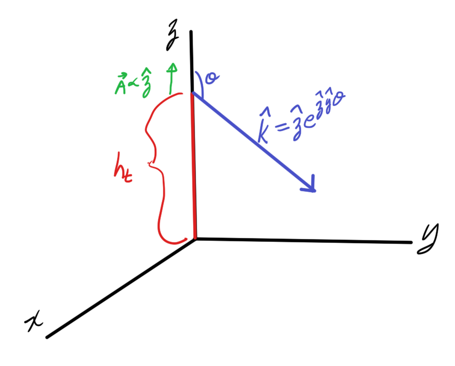
To understand these differences in reflection coefficients, consider first the field due to a vertical dipole as sketched in fig. 7, with a wave vector directed from the transmission point downwards in the z-y plane.

verticalDipoleConfigurationFig1

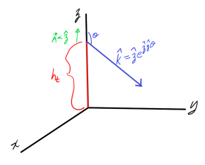
fig. 7. vertical dipole configuration.


The wave vector has direction

\begin{equation}\label{eqn:chapter4Notes:560}
\kcap = \zcap e^{\zcap \xcap \theta} = \zcap \cos\theta + \ycap \sin\theta.
\end{equation}

Suppose that the (magnetic) vector potential is that of an infinitesimal dipole

\begin{equation}\label{eqn:chapter4Notes:580}
\BA = \zcap \frac{\mu_0 I_0 l}{4 \pi r} e^{-j k r} %= \frac{A_r}{4 \pi r} e^{-j k r}
\end{equation}

The electric field, in the far field, can be computed by computing the normal projection to the wave vector direction

\begin{equation}\label{eqn:chapter4Notes:600}
\begin{aligned}
\BE
&= -j \omega \lr{\BA \wedge \kcap} \cdot \kcap \\
&= -j \omega \frac{\mu_0 I_0 l}{4 \pi r} \lr{\zcap \wedge \lr{\zcap \cos\theta
+ \ycap \sin\theta} } \lr{\zcap \cos\theta + \ycap \sin\theta} \\
&= -j \omega \frac{\mu_0 I_0 l}{4 \pi r} \lr{ \zcap \ycap \sin\theta }
\lr{\zcap \cos\theta + \ycap \sin\theta} \\
&= -j \omega \frac{\mu_0 I_0 l}{4 \pi r} \sin\theta \lr{-\ycap \cos\theta +
\zcap \sin\theta} \\
&= j \omega \frac{\mu_0 I_0 l}{4 \pi r} \sin\theta \ycap e^{\zcap \ycap \theta}.
\end{aligned}
\end{equation}

This is directed in the z-y plane rotated an additional \( \pi/2 \) past \( \kcap \). The magnetic field must then be directed into the page, along the x axis. This is sketched in fig. 8.

verticalDipoleConfigurationFig2

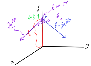
fig. 8. Electric and magnetic field directions


Referring to [2] (\eqntext 4.40) for the coefficient of reflection component

\begin{equation}\label{eqn:chapter4Notes:620}
R
=
\frac{
n_t \cos\theta_i – n_i \cos\theta_t
}
{
n_i \cos\theta_i + n_t \cos\theta_t
}
\end{equation}

This is the Fresnel equation for the case when
that corresponds to

\( \BE \) lies in the plane of incidence, and the magnetic field is completely parallel to the plane of reflection). For the no transmission case, allowing \( v_t \rightarrow 0 \), the index of refraction is \( n_t = c/v_t \rightarrow \infty \), and the reflection coefficient is \( 1 \) as claimed in section 4.7.2 of [1]. Because of the symmetry of this dipole configuration, the azimuthal angle that the wave vector is directed along does not matter.

Horizontal dipole reflection coefficient

In the class notes, a horizontal dipole coming out of the page is indicated. With the page representing the z-y plane, this is a magnetic vector potential directed along the x-axis direction

\begin{equation}\label{eqn:chapter4Notes:640}
\BA = \xcap \frac{\mu_0 I_0 l}{4 \pi r} e^{-j k r}.

\end{equation}

For a wave vector directed in the z-y plane as in \ref{eqn:chapter4Notes:560}, the electric far field is directed along

\begin{equation}\label{eqn:chapter4Notes:660}
\begin{aligned}
\lr{ \xcap \wedge \kcap } \cdot \kcap
&=
\xcap – \lr{ \xcap \cdot \kcap } \kcap \\
&=
\xcap – \lr{ \xcap \cdot \lr{
\zcap \cos\theta + \ycap \sin\theta
} } \kcap \\
&= \xcap.
\end{aligned}
\end{equation}

The electric far field lies completely in the plane of reflection. From [2] (\eqntext 4.34), the Fresnel reflection coefficients is

\begin{equation}\label{eqn:chapter4Notes:680}
R =
\frac{
n_i \cos\theta_i – n_t \cos\theta_t
}
{
n_i \cos\theta_i + n_t \cos\theta_t
},
\end{equation}

which approaches \( -1 \) when \( n_t \rightarrow \infty \). This is consistent with the image theorem summation that Prof. Eleftheriades used in class.

Azimuthal angle dependency of the reflection coefficient

Now consider a horizontal dipole directed along the y-axis. For the same wave vector direction as avove, the electric far field is now directed along

\begin{equation}\label{eqn:chapter4Notes:700}
\begin{aligned}
\lr{ \ycap \wedge \kcap } \cdot \kcap
&=
\ycap – \lr{ \ycap \cdot \kcap } \kcap \\
&=
\ycap – \lr{ \ycap \cdot \lr{
\zcap \cos\theta + \ycap \sin\theta
} } \kcap \\
&=
\ycap – \kcap \sin\theta \\
&=
\ycap – \sin\theta \lr{
\zcap \cos\theta + \ycap \sin\theta
} \\
&=
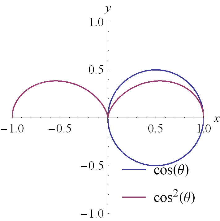
\ycap \cos^2 \theta – \sin\theta \cos\theta \zcap \\
&= \cos\theta \lr{ \ycap \cos\theta – \sin\theta \zcap } \\
&= \cos\theta \ycap e^{ \zcap \ycap \theta }.
\end{aligned}
\end{equation}

That is

\begin{equation}\label{eqn:chapter4Notes:720}
\BE =
-j \omega \frac{\mu_0 I_0 l}{4 \pi r} e^{-j k r}
\cos\theta \ycap e^{ \zcap \ycap \theta }.
\end{equation}

This far field electric field lies in the plane of incidence (a direction of \( \thetacap \) rotated by \( \pi/2 \)), not in the plane of reflection. The corresponding magnetic field should be directed along the plane of reflection, which is easily confirmed by calculation

\begin{equation}\label{eqn:chapter4Notes:740}
\begin{aligned}
\kcap \cross
\lr{ \ycap \cos\theta – \sin\theta \zcap }
&=
\lr{ \zcap \cos\theta + \ycap \sin\theta } \cross
\lr{ \ycap \cos\theta – \sin\theta \zcap } \\
&=
-\xcap \cos^2 \theta – \xcap \sin^2\theta \\
&= -\xcap.
\end{aligned}
\end{equation}

The far field magnetic field is seen to be

\begin{equation}\label{eqn:chapter4Notes:721}
\BH =
j \omega \frac{I_0 l}{4 \pi r} e^{-j k r}
\cos\theta \xcap,
\end{equation}

so a reflection coefficient of \( 1 \) is required to calculate the power loss after a single ground reflection signal bounce for this relative orientation of antenna to the target.

I fail to see how the horizontal dipole treatment in section 4.7.5 can use a single reflection coefficient without taking into account the azimuthal dependency of that reflection coefficient.

References

[1] Constantine A Balanis. Antenna theory: analysis and design. John Wiley \& Sons, 3rd edition, 2005.

[2] E. Hecht. Optics. 1998.

[3] JD Jackson. Classical Electrodynamics. John Wiley and Sons, 2nd edition, 1975.

[4] Wikipedia. Magnetic potential — Wikipedia, The Free Encyclopedia, 2015. URL https://en.wikipedia.org/w/index.php?title=Magnetic_potential&oldid=642387563. [Online; accessed 5-February-2015].

Notes for ece1229 antenna theory

February 4, 2015 ece1229 , , , , , , , , , , , , , , , , , , , , , , , , , , , , , , , , , , , , , , , , , , , , , , , , , , , , , , , , , , , , , , , , , , , , , , , , , , , , , , , , , , , ,

I’ve now posted a first set of notes for the antenna theory course that I am taking this term at UofT.

Unlike most of the other classes I have taken, I am not attempting to take comprehensive notes for this class. The class is taught on slides that match the textbook so closely, there is little value to me taking notes that just replicate the text. Instead, I am annotating my copy of textbook with little details instead. My usual notes collection for the class will contain musings of details that were unclear, or in some cases, details that were provided in class, but are not in the text (and too long to pencil into my book.)

The notes linked above include:

  • Reading notes for chapter 2 (Fundamental Parameters of Antennas) and chapter 3 (Radiation Integrals and Auxiliary Potential Functions) of the class text.
  • Geometric Algebra musings.  How to do formulate Maxwell’s equations when magnetic sources are also included (those modeling magnetic dipoles).
  • Some problems for chapter 2 content.

Fundamental parameters of antennas

January 22, 2015 ece1229 , , , , , , , , , , , , , , , , , , , , , , , , , , , , , , , , , ,

[Click here for a PDF of this post with nicer formatting]

This is my first set of notes for the UofT course ECE1229, Advanced Antenna Theory, taught by Prof. Eleftheriades, covering ch. 2 [1] content.

Unlike most of the other classes I have taken, I am not attempting to take comprehensive notes for this class. The class is taught on slides that match the textbook so closely, there is little value to me taking notes that just replicate the text. Instead, I am annotating my copy of textbook with little details instead. My usual notes collection for the class will contain musings of details that were unclear, or in some cases, details that were provided in class, but are not in the text (and too long to pencil into my book.)

Poynting vector

The Poynting vector was written in an unfamiliar form

\begin{equation}\label{eqn:chapter2Notes:560}
\boldsymbol{\mathcal{W}} = \boldsymbol{\mathcal{E}} \cross \boldsymbol{\mathcal{H}}.
\end{equation}

I can roll with the use of a different symbol (i.e. not \(\BS\)) for the Poynting vector, but I’m used to seeing a \( \frac{c}{4\pi} \) factor ([6] and [5]). I remembered something like that in SI units too, so was slightly confused not to see it here.

Per [3] that something is a \( \mu_0 \), as in

\begin{equation}\label{eqn:chapter2Notes:580}
\boldsymbol{\mathcal{W}} = \inv{\mu_0} \boldsymbol{\mathcal{E}} \cross \boldsymbol{\mathcal{B}}.
\end{equation}

Note that the use of \( \boldsymbol{\mathcal{H}} \) instead of \( \boldsymbol{\mathcal{B}} \) is what wipes out the requirement for the \( \frac{1}{\mu_0} \) term since \( \boldsymbol{\mathcal{H}} = \boldsymbol{\mathcal{B}}/\mu_0 \), assuming linear media, and no magnetization.

Typical far-field radiation intensity

It was mentioned that

\begin{equation}\label{eqn:advancedantennaL1:20}
U(\theta, \phi)
=
\frac{r^2}{2 \eta_0} \Abs{ \BE( r, \theta, \phi) }^2
=
\frac{1}{2 \eta_0} \lr{ \Abs{ E_\theta(\theta, \phi) }^2 + \Abs{ E_\phi(\theta, \phi) }^2},
\end{equation}

where the intrinsic impedance of free space is

\begin{equation}\label{eqn:advancedantennaL1:480}
\eta_0 = \sqrt{\frac{\mu_0}{\epsilon_0}} = 377 \Omega.
\end{equation}

(this is also eq. 2-19 in the text.)

To get an understanding where this comes from, consider the far field radial solutions to the electric and magnetic dipole problems, which have the respective forms (from [3]) of

\begin{equation}\label{eqn:chapter2Notes:740}
\begin{aligned}
\boldsymbol{\mathcal{E}} &= -\frac{\mu_0 p_0 \omega^2 }{4 \pi } \frac{\sin\theta}{r} \cos\lr{w t – k r} \thetacap \\
\boldsymbol{\mathcal{B}} &= -\frac{\mu_0 p_0 \omega^2 }{4 \pi c} \frac{\sin\theta}{r} \cos\lr{w t – k r} \phicap \\
\end{aligned}
\end{equation}
\begin{equation}\label{eqn:chapter2Notes:760}
\begin{aligned}
\boldsymbol{\mathcal{E}} &= \frac{\mu_0 m_0 \omega^2 }{4 \pi c} \frac{\sin\theta}{r} \cos\lr{w t – k r} \phicap \\
\boldsymbol{\mathcal{B}} &= -\frac{\mu_0 m_0 \omega^2 }{4 \pi c^2} \frac{\sin\theta}{r} \cos\lr{w t – k r} \thetacap \\
\end{aligned}
\end{equation}

In neither case is there a component in the direction of propagation, and in both cases (using \( \mu_0 \epsilon_0 = 1/c^2\))

\begin{equation}\label{eqn:chapter2Notes:780}
\Abs{\boldsymbol{\mathcal{H}}}
= \frac{\Abs{\boldsymbol{\mathcal{E}}}}{\mu_0 c}
= \Abs{\boldsymbol{\mathcal{E}}} \sqrt{\frac{\epsilon_0}{\mu_0}}
= \inv{\eta_0}\Abs{\boldsymbol{\mathcal{E}}} .
\end{equation}

A superposition of the phasors for such dipole fields, in the far field, will have the form

\begin{equation}\label{eqn:chapter2Notes:800}
\begin{aligned}
\BE &= \inv{r} \lr{ E_\theta(\theta, \phi) \thetacap + E_\phi(\theta, \phi) \phicap } \\
\BB &= \inv{r c} \lr{ E_\theta(\theta, \phi) \thetacap – E_\phi(\theta, \phi) \phicap },
\end{aligned}
\end{equation}

with a corresponding time averaged Poynting vector

\begin{equation}\label{eqn:chapter2Notes:820}
\begin{aligned}
\BW_{\textrm{av}}
&= \inv{2 \mu_0} \BE \cross \BB^\conj \\
&=
\inv{2 \mu_0 c r^2}
\lr{ E_\theta \thetacap + E_\phi \phicap } \cross
\lr{ E_\theta^\conj \thetacap – E_\phi^\conj \phicap } \\
&=
\frac{\thetacap \cross \phicap}{2 \mu_0 c r^2}
\lr{ \Abs{E_\theta}^2 + \Abs{E_\phi}^2 } \\
&=
\frac{\rcap}{2 \eta_0 r^2}
\lr{ \Abs{E_\theta}^2 + \Abs{E_\phi}^2 },
\end{aligned}
\end{equation}

verifying \ref{eqn:advancedantennaL1:20} for a superposition of electric and magnetic dipole fields. This can likely be shown for more general fields too.

Field plots

We can plot the fields, or intensity (or log plots in dB of these).
It is pointed out in [3] that when there is \( r \) dependence these plots are done by considering the values of at fixed \( r \).

The field plots are conceptually the simplest, since that vector parameterizes
a surface. Any such radial field with magnitude \( f(r, \theta, \phi) \) can
be plotted in Mathematica in the \( \phi = 0 \) plane at \( r = r_0 \), or in
3D (respectively, but also at \( r = r_0\)) with code like that of the
following listing

ParametricPlotListing

Intensity plots can use the same code, with the only difference being the interpretation. The surface doesn’t represent the value of a vector valued radial function, but is the magnitude of a scalar valued function evaluated at \( f( r_0, \theta, \phi) \).

The surfaces for \( U = \sin\theta, \sin^2\theta \) in the plane are parametrically plotted in fig. 2, and for cosines in fig. 1 to compare with textbook figures.

CoSineAndCoSineSqFig1pn

fig 1. Cosinusoidal radiation intensities

SineAndSinSqFig3pn

fig 2. Sinusoidal radiation intensities


Visualizations of \( U = \sin^2 \theta\) and \( U = \cos^2 \theta\) can be found in fig. 3 and fig. 4 respectively. Even for such simple functions these look pretty cool.

SineSq3DFig4pn

fig 3. Square sinusoidal radiation intensity


CoSineSq3DFig2pn

fig 4. Square cosinusoidal radiation intensity


dB vs dBi

Note that dBi is used to indicate that the gain is with respect to an “isotropic” radiator.
This is detailed more in [2].

Trig integrals

Tables 1.1 and 1.2 produced with tableOfTrigIntegrals.nb have some of the sine and cosine integrals that are pervasive in this chapter.

trigIntegralsUpToPiBy2

trigIntegralsUpToPi

Polarization vectors

The text introduces polarization vectors \( \rhocap \) , but doesn’t spell out their form. Consider a plane wave field of the form

\begin{equation}\label{eqn:chapter2Notes:840}
\BE
=
E_x e^{j \phi_x} e^{j \lr{ \omega t – k z }} \xcap
+
E_y e^{j \phi_y} e^{j \lr{ \omega t – k z }} \ycap.
\end{equation}

The \( x, y \) plane directionality of this phasor can be written

\begin{equation}\label{eqn:chapter2Notes:860}
\Brho =
E_x e^{j \phi_x} \xcap
+
E_y e^{j \phi_y} \ycap,
\end{equation}

so that

\begin{equation}\label{eqn:chapter2Notes:880}
\BE = \Brho e^{j \lr{ \omega t – k z }}.
\end{equation}

Separating this direction and magnitude into factors

\begin{equation}\label{eqn:chapter2Notes:900}
\Brho = \Abs{\BE} \rhocap,
\end{equation}

allows the phasor to be expressed as

\begin{equation}\label{eqn:chapter2Notes:920}
\BE = \rhocap \Abs{\BE} e^{j \lr{ \omega t – k z }}.
\end{equation}

As an example, suppose that \( E_x = E_y \), and set \( \phi_x = 0 \). Then

\begin{equation}\label{eqn:chapter2Notes:940}
\rhocap = \xcap + \ycap e^{j \phi_y}.
\end{equation}

Phasor power

In section 2.13 the phasor power is written as

\begin{equation}\label{eqn:chapter2Notes:620}
I^2 R/2,
\end{equation}

where \( I, R \) are the magnitudes of phasors in the circuit.

I vaguely recall this relation, but had to refer back to [4] for the details.
This relation expresses average power over a period associated with the frequency of the phasor

\begin{equation}\label{eqn:chapter2Notes:640}
\begin{aligned}
P
&= \inv{T} \int_{t_0}^{t_0 + T} p(t) dt \\
&= \inv{T} \int_{t_0}^{t_0 + T} \Abs{\BV} \cos\lr{ \omega t + \phi_V }
\Abs{\BI} \cos\lr{ \omega t + \phi_I} dt \\
&= \inv{T} \int_{t_0}^{t_0 + T} \Abs{\BV} \Abs{\BI}
\lr{
\cos\lr{ \phi_V – \phi_I } + \cos\lr{ 2 \omega t + \phi_V + \phi_I}
}
dt \\
&= \inv{2} \Abs{\BV} \Abs{\BI} \cos\lr{ \phi_V – \phi_I }.
\end{aligned}
\end{equation}

Introducing the impedance for this circuit element

\begin{equation}\label{eqn:chapter2Notes:660}
\BZ = \frac{ \Abs{\BV} e^{j\phi_V} }{ \Abs{\BI} e^{j\phi_I} } = \frac{\Abs{\BV}}{\Abs{\BI}} e^{j\lr{\phi_V – \phi_I}},
\end{equation}

this average power can be written in phasor form

\begin{equation}\label{eqn:chapter2Notes:680}
\BP = \inv{2} \Abs{\BI}^2 \BZ,
\end{equation}

with
\begin{equation}\label{eqn:chapter2Notes:700}
P = \textrm{Re} \BP.
\end{equation}

Observe that we have to be careful to use the absolute value of the current phasor \( \BI \), since \( \BI^2 \) differs in phase from \( \Abs{\BI}^2 \). This explains the conjugation in the [4] definition of complex power, which had the form

\begin{equation}\label{eqn:chapter2Notes:720}
\BS = \BV_{\textrm{rms}} \BI^\conj_{\textrm{rms}}.
\end{equation}

Radar cross section examples

Flat plate.

\begin{equation}\label{eqn:chapter2Notes:960}
\sigma_{\textrm{max}} = \frac{4 \pi \lr{L W}^2}{\lambda^2}
\end{equation}

RCSsquareGeometryFig1

fig. 6. Square geometry for RCS example.


Sphere.

In the optical limit the radar cross section for a sphere

RCSsphereGeometryFig3

fig. 7. Sphere geometry for RCS example.


\begin{equation}\label{eqn:chapter2Notes:980}
\sigma_{\textrm{max}} = \pi r^2
\end{equation}

Note that this is smaller than the physical area \( 4 \pi r^2 \).

Cylinder.

RCScylinderGeometryFig1

fig. 8. Cylinder geometry for RCS example.


\begin{equation}\label{eqn:chapter2Notes:1000}
\sigma_{\textrm{max}} = \frac{ 2 \pi r h^2}{\lambda}
\end{equation}

Tridedral corner reflector

trihedralCornerReflectorFig6

fig. 9. Trihedral corner reflector geometry for RCS example.


\begin{equation}\label{eqn:chapter2Notes:1020}
\sigma_{\textrm{max}} = \frac{ 4 \pi L^4}{3 \lambda^2}
\end{equation}

Scattering from a sphere vs frequency

Frequency dependence of spherical scattering is sketched in fig. 10.

  • Low frequency (or small particles): Rayleigh\begin{equation}\label{eqn:chapter2Notes:1040}
    \sigma = \lr{\pi r^2} 7.11 \lr{\kappa r}^4, \qquad \kappa = 2 \pi/\lambda.
    \end{equation}
  • Mie scattering (resonance),\begin{equation}\label{eqn:chapter2Notes:1060}
    \sigma_{\textrm{max}}(A) = 4 \pi r^2
    \end{equation}
    \begin{equation}\label{eqn:chapter2Notes:1080}
    \sigma_{\textrm{max}}(B) = 0.26 \pi r^2.
    \end{equation}
  • optical limit ( \(r \gg \lambda\) )\begin{equation}\label{eqn:chapter2Notes:1100}
    \sigma = \pi r^2.
    \end{equation}
sphericalScatteringFig5

fig 10. Scattering from a sphere vs frequency (from Prof. Eleftheriades’ class notes).

FIXME: Do I have a derivation of this in my optics notes?

Notation

  • Time average.
    Both Prof. Eleftheriades
    and the text [1] use square brackets \( [\cdots] \) for time averages, not \( <\cdots> \). Was that an engineering convention?
  • Prof. Eleftheriades
    writes \(\Omega\) as a circle floating above a face up square bracket, as in fig. 1, and \( \sigma \) like a number 6, as in fig. 1.
  • Bold vectors are usually phasors, with (bold) calligraphic script used for the time domain fields. Example: \( \BE(x,y,z,t) = \ecap E(x,y) e^{j \lr{\omega t – k z}}, \boldsymbol{\mathcal{E}}(x, y, z, t) = \textrm{Re} \BE \).
greekStyleOmegaFig1

fig. 11. Prof. handwriting decoder ring: Omega

sigmaFig1

fig 12. Prof. handwriting decoder ring: sigma


References

[1] Constantine A Balanis. Antenna theory: analysis and design. John Wiley \& Sons, 3rd edition, 2005.

[3] David Jeffrey Griffiths and Reed College. Introduction to electrodynamics. Prentice hall Upper Saddle River, NJ, 3rd edition, 1999.

[4] J.D. Irwin. Basic Engineering Circuit Analysis. MacMillian, 1993.

[5] JD Jackson. Classical Electrodynamics. John Wiley and Sons, 2nd edition, 1975.

[6] L.D. Landau and E.M. Lifshitz. The classical theory of fields. Butterworth-Heinemann, 1980. ISBN 0750627689.