impedance

Impedance refresher.

March 21, 2025 math and physics play , , , , , , , , , , , ,

[Click here for a PDF version of this post]

Karl is taking his circuits course right now, which means that I get a chance to field some questions. I don’t get an excuse to think about this stuff any more. It’s fun material, since most of the ideas are all really simple, and you can figure out everything from first principles.

Karl just started sinusoidal circuits, which I think is a bit exciting. They are such a nice special case, as complex calculations are all effectively reduced to \( V = I R \) style computations.

Solving RLC circuits for general time dependent sources.

To contrast the simple case of sinusoidal sources, let’s consider what we have to do in order to solve a general case RLC circuit. The simple basic RC circuit sketched in fig. 1 provides a good illustrative example, even though it does not include any inductance.

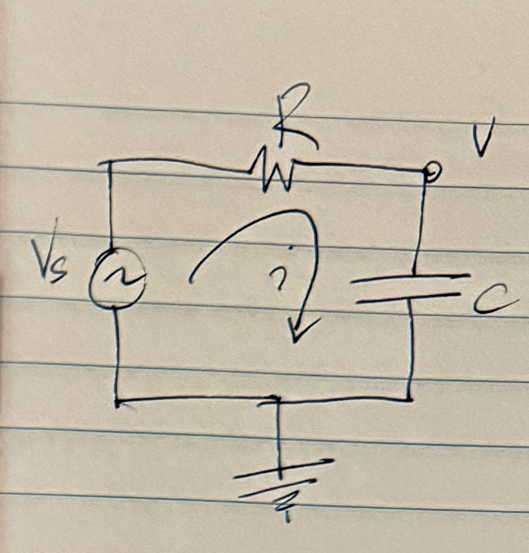
With \( v \) as the voltage at the capacitor, the equations that describe the circuit are
\begin{equation}\label{eqn:impedance:20}
\begin{aligned}
v_s – v &= i R \\
i &= C \frac{dv}{dt}.
\end{aligned}
\end{equation}

We can combine these into one equation for \( v \). Letting \( \tau = RC \), that is
\begin{equation}\label{eqn:impedance:40}
v + \tau \frac{dv}{dt} = v_s.
\end{equation}
Here \( v_s = v_s(t) \) can be an arbitrary function of time. This is a simple enough differential equation, and can probably be solved in various ways (integrating factors, Fourier transforms, Laplace transforms, …)

For illustration purposes, let’s tackle this little equation with Fourier transforms, a method logically equivalent to the computation of the Green’s function for the system.

Let’s use a symmetric representation of the Fourier transform
\begin{equation}\label{eqn:impedance:60}
\begin{aligned}
F(\omega) &= \inv{\sqrt{2 \pi}} \int_{-\infty}^\infty e^{-j\omega t} f(t) dt \\
f(t) &= \inv{\sqrt{2 \pi}} \int_{-\infty}^\infty e^{j\omega t} F(\omega) d\omega \\
\end{aligned}
\end{equation}
Recall that the Fourier transform of the derivative is just a \( j \omega \) scaled frequency domain function, which we show with integration by parts
\begin{equation}\label{eqn:impedance:80}
\begin{aligned}
\inv{\sqrt{2 \pi}} \int_{-\infty}^\infty e^{-j\omega t} \frac{df}{dt} dt
&= \inv{\sqrt{2 \pi}} \int_{-\infty}^\infty \lr{ \frac{d}{dt} \lr{ f(t) e^{-j \omega t} } – f(t) \frac{d}{dt}\lr{ e^{-j\omega t}} } dt \\
&= j \omega F(\omega).
\end{aligned}
\end{equation}
That means that the frequency domain equivalent of our system is
\begin{equation}\label{eqn:impedance:100}
V + j \omega \tau V = V_s,
\end{equation}
or
\begin{equation}\label{eqn:impedance:120}
V(\omega) = \frac{V_s(\omega)}{1 + j \omega \tau}.
\end{equation}
Inverse transformation yields
\begin{equation}\label{eqn:impedance:140}
\begin{aligned}
v(t)
&= \inv{\sqrt{2 \pi}} \int_{-\infty}^\infty e^{j\omega t} \frac{V_s(\omega)}{1 + j \omega \tau} d\omega \\
&= \inv{2 \pi} \iint_{-\infty}^\infty e^{j\omega t} \frac{1}{1 + j \omega \tau} d\omega e^{-j\omega t’} v_s(t’) dt’ \\
&= \int_{-\infty}^\infty dt’ v_s(t’) \inv{2\pi} \int_{-\infty}^\infty \frac{e^{j\omega(t-t’)}}{1 + j \omega \tau} d\omega,
\end{aligned}
\end{equation}
or with
\begin{equation}\label{eqn:impedance:160}
G(u) = \inv{2\pi} \int_{-\infty}^\infty \frac{e^{j\omega u}}{1 + j \omega \tau} d\omega,
\end{equation}
\begin{equation}\label{eqn:impedance:180}
v(t) = \int_{-\infty}^\infty v_s(t’) G(t – t’) dt’.
\end{equation}
We just need to evaluate the Green’s function \( G(u) \) to proceed, which we can do with standard contour integration, first writing:

\begin{equation}\label{eqn:impedance:200}
\begin{aligned}
G(u)
&= \inv{2\pi j \tau} \int_{-\infty}^\infty \frac{e^{j\omega u}}{\inv{j\tau} + \omega} d\omega \\
&= \inv{2\pi j \tau} \oint \frac{e^{j z u}}{\inv{j\tau} + z} dz.
\end{aligned}
\end{equation}
This has a single pole at \( z = j/\tau \). We need an infinite semicircular contour in the lower half plane for \( u < 0 \), and can use the upper half plane infinite semicircular contour (surrounding the pole) for \( u > 0 \). That gives
\begin{equation}\label{eqn:impedance:220}
\begin{aligned}
G(u)
&= \Theta(u) \frac{2 \pi j}{2\pi j \tau} \evalbar{e^{j z u}}{z = j/\tau} \\
&= \frac{\Theta(u)}{\tau} e^{- u/\tau}.
\end{aligned}
\end{equation}

The solution to the problem, for any Fourier integrable source \( v_s(t) \), is
\begin{equation}\label{eqn:impedance:240}
\boxed{
v(t) = \int_{-\infty}^t v_s(t’) \frac{e^{- \lr{t – t’}/\tau}}{\tau} dt’.
}
\end{equation}

As a check, let’s evaluate this convolution integral for a step source \( v_s(t) = V \Theta(t) \), to find
\begin{equation}\label{eqn:impedance:260}
\begin{aligned}
v(t)
&= \frac{V e^{-t/tau}}{\tau} \int_0^t e^{t’/\tau} dt’ \\
&= V e^{-t/tau} \evalrange{e^{t’/\tau} }{0}{t} \\
&= V e^{-t/tau} \lr{ e^{t/\tau} – 1 } \\
&= V \lr{ 1 – e^{-t/\tau} }.
\end{aligned}
\end{equation}
This is the damped time domain response that we remember for an RC circuit. In Karl’s first year engineering notes, this was presented as a given (without the step factor), and he had to verify that it worked by differentiation (for \( t > 0 \).)

Solving this exactly, even for arbitrary sources, as we’ve done above, is not strictly hard, if you have all the required tools. But the first year engineering student doesn’t have all those tools to start with. This is where the beauty of the phasor techniques for sinusoidal sources comes in. Let’s now see how that works.

Phasor approach.

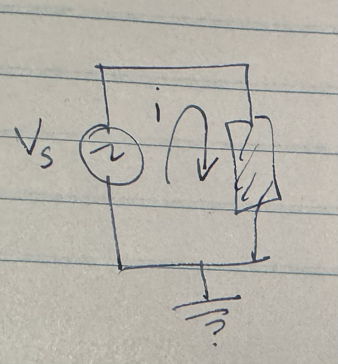
Let’s consider the three simplest RLC circuits, each with just a single element, and a variable voltage source. I’ll depict that element with a box as in fig. 2.

Resistor case.

If the element is a resistor with value \( R \), our equations are simple
\begin{equation}\label{eqn:impedance:280}
v_s = i R.
\end{equation}
Clearly \( i \) is directly proportional to the source voltage. In particular, if \( v_s(t) \) has a sinusoidal character, such as
\begin{equation}\label{eqn:impedance:300}
v_s(t) = V \cos(\omega t),
\end{equation}
then
\begin{equation}\label{eqn:impedance:320}
i(t) = \frac{V}{R} \cos\lr{ \omega t }.
\end{equation}
In particular, if we let \( i(t) = I \cos\lr{ \omega t } \), then we have
\begin{equation}\label{eqn:impedance:340}
I = \frac{V}{R},
\end{equation}
or \( V = I R \).

Capacitor case.

If the load element is a capacitor with capacitance \( C \), then the equation for the system is
\begin{equation}\label{eqn:impedance:360}
i = C \frac{dv_s(t)}{dt}.
\end{equation}
If we just plug in \( v_s(t) = V \cos(\omega t) \), as before, we get a bit of a mess
\begin{equation}\label{eqn:impedance:380}
i = -C \omega V \sin\lr{ \omega t }.
\end{equation}
We no longer have a nice simple proportionality relationship between the current and the voltage source, as the capacitor has introduced a phase shift into the mix.
We can figure out that phase factor by solving the equation
\begin{equation}\label{eqn:impedance:400}
-\sin x = \cos\lr{ x + \phi }.
\end{equation}
The easiest way to solve this is to express the sinusoids in complex exponential form
\begin{equation}\label{eqn:impedance:420}
\textrm{Re} \lr{ e^{j + \phi} } = \Real \lr{ j e^{j x} } = \Real \lr{ e^{j \pi/2} e^{j x} }.
\end{equation}
We see that the phase factor is a \( \pi/2 \) shift. However, even better, we have a strong hint that working with complex exponentials may be a better approach to formulating the problem.

Let’s write
\begin{equation}\label{eqn:impedance:440}
v_s(t) = V \cos\lr{ \omega t } = \textrm{Re} \lr{ V e^{j \omega t} }.
\end{equation}
Then we have
\begin{equation}\label{eqn:impedance:460}
i(t) = C V \textrm{Re} \lr{ \frac{d}{dt} e^{j \omega t} }.
\end{equation}
If we also assume that we can write
\begin{equation}\label{eqn:impedance:480}
i(t) = \textrm{Re} \lr{ I e^{j \omega t} },
\end{equation}
then if the real parts are equal, we must also have
\begin{equation}\label{eqn:impedance:500}
I e^{j \omega t} = j \omega C V e^{j \omega t},
\end{equation}
or
\begin{equation}\label{eqn:impedance:520}
I = j \omega C V.
\end{equation}
We have a \( V = I R \) relationship, which we write as
\begin{equation}\label{eqn:impedance:540}
V = I Z,
\end{equation}
where
\begin{equation}\label{eqn:impedance:560}
Z = \inv{j \omega C}.
\end{equation}
This is the phasor description of the circuit.

Inductive case.

If the circuit has an inductive load, then the system equation is
\begin{equation}\label{eqn:impedance:580}
v_s(t) = L \frac{di}{dt}.
\end{equation}
Again, we can write \( v_s(t) = \textrm{Re} \lr{ V e^{j\omega t} } \), and assume that \( i = \Real \lr{ I e^{j\omega t} } \). We then require
\begin{equation}\label{eqn:impedance:600}
V e^{j \omega t} = L \frac{d}{dt} \lr{ I e^{j \omega t} },
\end{equation}
or
\begin{equation}\label{eqn:impedance:620}
V = j \omega L I.
\end{equation}
We write
\begin{equation}\label{eqn:impedance:640}
Z = j \omega L,
\end{equation}
so once again \( V = I Z \).

Solving a more complex RLC configuration.

An example of a more complicated RLC circuit is sketched in fig. 3.

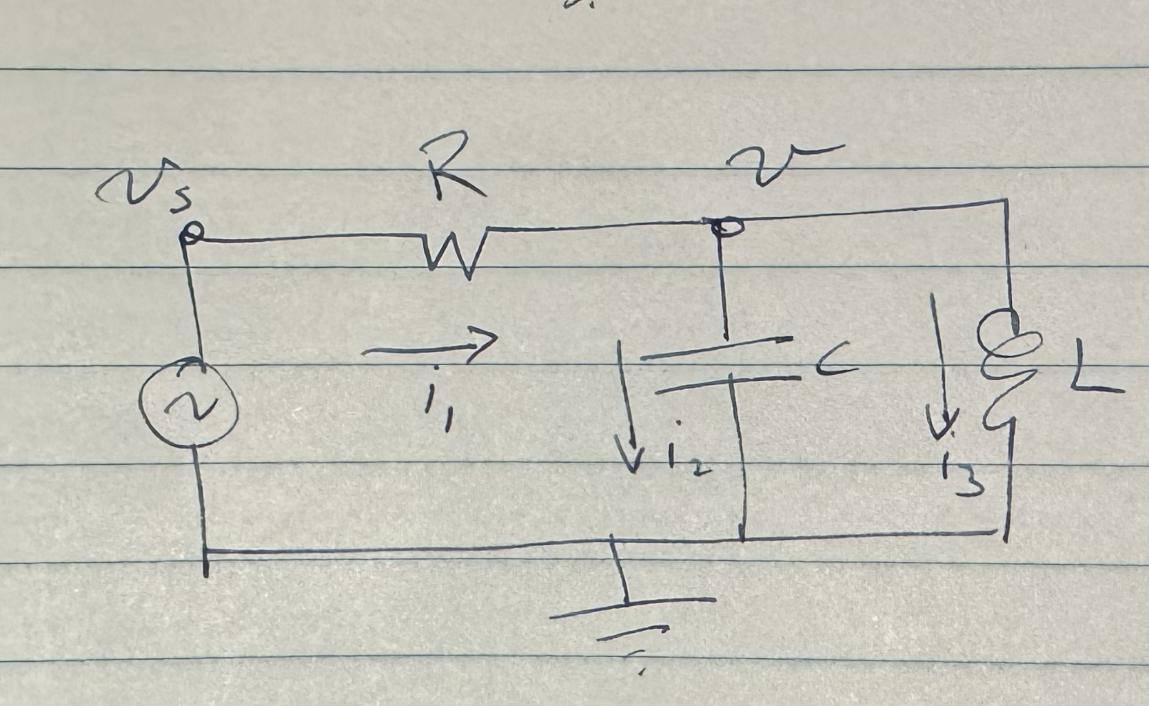
Here we have two impedances in parallel
\begin{equation}\label{eqn:impedance:660}
\begin{aligned}
Z_C &= \inv{j \omega C} \\
Z_L &= j \omega L.
\end{aligned}
\end{equation}
The parallel impedance through that reactive load is
\begin{equation}\label{eqn:impedance:680}
\begin{aligned}
Z
&= \lr{ \inv{Z_C} + \inv{Z_L} }^{-1} \\
&= \lr{ j \omega C + \inv{ j \omega L } }^{-1}.
\end{aligned}
\end{equation}
We can compute the current through \( R \) now
\begin{equation}\label{eqn:impedance:700}
I = \frac{V_s}{ R + \lr{ j \omega C + \inv{ j \omega L } }^{-1} }.
\end{equation}
We also have
\begin{equation}\label{eqn:impedance:720}
\frac{V_s – V}{R} = I,
\end{equation}
or
\begin{equation}\label{eqn:impedance:740}
\begin{aligned}
V
&= V_s – I R \\
&= V_s \lr{ 1 – \frac{R}{ R + \lr{ j \omega C + \inv{ j \omega L } }^{-1} } } \\
&= V_s \frac{\lr{ j \omega C + \inv{ j \omega L } }^{-1} }{ R + \lr{ j \omega C + \inv{ j \omega L } }^{-1} } \\
&= \frac{V_s}{ R \lr{ j \omega C + \inv{ j \omega L } } + 1 }.
\end{aligned}
\end{equation}
The complicated time response for this system is reduced to a trivial voltage divider calculation. We see that it was kind of pointless to run an inductor and capacitor in parallel, as they are both purely reactive (imaginary). That’s a detail that I didn’t remember, since it’s been decades since I did any practical circuits applications. However, the point is, by using a complex exponential source representation, these types of systems are reduced from systems of coupled differential equations to simple linear systems. Imagine how messy it would be to try to solve this system using the Green’s function methods that we used above!

ECE1236H Microwave and Millimeter-Wave Techniques. Lecture 7: Multisection quarter-wavelength transformers. Taught by Prof. G.V. Eleftheriades

February 11, 2016 ece1236 , , , , , , ,

[Click here for a PDF of this post with nicer formatting] or [Click here for my notes compilation for this class]

Disclaimer

Peeter’s lecture notes from class. These may be incoherent and rough.

These are notes for the UofT course ECE1236H, Microwave and Millimeter-Wave Techniques, taught by Prof. G.V. Eleftheriades, covering ch 5. [3] content.

Terminology review

\begin{equation}\label{eqn:uwavesDeck7MultisectionTransformersCore:20}
Z_{\textrm{in}} = R + j X
\end{equation}
\begin{equation}\label{eqn:uwavesDeck7MultisectionTransformersCore:40}
Y_{\textrm{in}} = G + j B
\end{equation}

  • \( Z_{\textrm{in}} \) : impedance
  • \( R \) : resistance
  • \( X \) : reactance
  • \( Y_{\textrm{in}} \) : admittance
  • \( G \) : conductance
  • \( B \) : susceptance

Apparently this notation goes all the way back to Heavyside!

Multisection transformers

Using a transformation of the form fig. 1 it is possible to optimize for maximum power delivery, using for example a matching transformation \( Z_{\textrm{in}} = Z_1^2/R_{\textrm{L}} = Z_0\), or \( Z_1 = \sqrt{R_{\textrm{L}} Z_0} \). Unfortunately, such a transformation does not allow any control over the bandwidth. This results in a pinched frequency response for which the standard solution is to add more steps as sketched in fig. 2.

../../figures/ece1236/Feb10Fig2: fig. 2. Pinched frequency response.
../../figures/ece1236/deck7Fig1: fig. 3. Single and multiple stage impedance matching.

This can be implemented in electronics, or potentially geometrically as in this sketch of a microwave stripline transformer implementation fig. 3.

../../figures/ece1236/deck7Fig3: fig. 3. Stripline implementation of staged impedance matching.

To find a multistep transformation algebraically can be hard, but it is easy to do on a Smith chart. The rule of thumb is that we want to stay near the center of the chart with each transformation.

There is however, a closed form method of calculating a specific sort of multisection transformation that is algebraically tractable. That method uses a chain of \( \lambda/4 \) transformers to increase the bandwidth as sketched in fig. 4.

../../figures/ece1236/deck7Fig4: fig. 4. Multiple \( \lambda/4 \) transformers.

The total reflection coefficient can be approximated to first order by summing the reflections at each stage (without considering there may be other internal reflections of transmitted field components). Algebraically that is

\begin{equation}\label{eqn:uwavesDeck7MultisectionTransformersCore:60}
\Gamma(\Theta) \approx \Gamma_0
+ \Gamma_1 e^{-2 j \Theta} +
+ \Gamma_2 e^{-4 j \Theta} + \cdots
+ \Gamma_N e^{-2 N j \Theta},
\end{equation}

where

\begin{equation}\label{eqn:uwavesDeck7MultisectionTransformersCore:80}
\Gamma_n = \frac{Z_{n+1} – Z_n}{Z_{n+1} + Z_n}
\end{equation}

Why? Consider reflections at the Z_1, Z_2 interface as sketched in fig. 5.

../../figures/ece1236/deck7Fig5: fig. 5. Single stage of multiple \( \lambda/4\) transformers.

Assuming small reflections, where \( \Abs{\Gamma} \ll 1 \) then \( T = 1 + \Gamma \approx 1 \). Here

\begin{equation}\label{eqn:uwavesDeck7MultisectionTransformersCore:100}
\begin{aligned}
\Theta
&= \beta l \\
&= \frac{2 \pi}{\lambda} \frac{\lambda}{4} \\
&= \frac{\pi}{2}.
\end{aligned}
\end{equation}

at the design frequency \( \omega_0 \). We assume that \( Z_n \) are either monotonically increasing if \( R_{\textrm{L}} > Z_0 \), or decreasing if \( R_{\textrm{L}} < Z_0 \).

Binomial multisection transformers

Let

\begin{equation}\label{eqn:uwavesDeck7MultisectionTransformersCore:120}
\Gamma(\Theta) = A \lr{ 1 + e^{-2 j \Theta} }^N
\end{equation}

This type of a response is maximally flat, and is plotted in fig. 1.
../../figures/ece1236/multitransformerFig1: fig. 1. Binomial transformer.

The absolute value of the reflection coefficient is

\begin{equation}\label{eqn:uwavesDeck7MultisectionTransformersCore:160}
\begin{aligned}
\Abs{\Gamma(\Theta)}
&=
\Abs{A} \lr{ e^{j \Theta} + e^{- j \Theta} }^N \\
&=
2^N \Abs{A} \cos^N\Theta.
\end{aligned}
\end{equation}

When \( \Theta = \pi/2 \) this is clearly zero. It’s derivatives are

\begin{equation}\label{eqn:uwavesDeck7MultisectionTransformersCore:180}
\begin{aligned}
\frac{d \Abs{\Gamma}}{d\Theta} &= -N \cos^{N-1} \Theta \sin\Theta \\
\frac{d^2 \Abs{\Gamma}}{d\Theta^2} &= -N \cos^{N-1} \Theta \cos\Theta N(N-1) \cos^{N-2} \Theta \sin\Theta \\
\frac{d^3 \Abs{\Gamma}}{d\Theta^3} &= \cdots
\end{aligned}
\end{equation}

There is a \( \cos^{N-k} \) term for all derivatives \( d^k/d\Theta^k \) where \( k \le N-1 \), so for an N-section transformer

\begin{equation}\label{eqn:uwavesDeck7MultisectionTransformersCore:140}
\frac{d^n}{d\Theta^n} \Abs{\Gamma(\Theta)}_{\omega_0} = 0,
\end{equation}

for \( n = 1, 2, \cdots, N-1 \). The constant \( A \) is determined by the limit \( \Theta \rightarrow 0 \), so

\begin{equation}\label{eqn:uwavesDeck7MultisectionTransformersCore:200}
\Gamma(0) = 2^N A = \frac{Z_{\textrm{L}} – Z_0}{Z_{\textrm{L}} + Z_0},
\end{equation}

because the various \( \Theta \) sections become DC wires when the segment length goes to zero. This gives

\begin{equation}\label{eqn:uwavesDeck7MultisectionTransformersCore:220}
\boxed{
A = 2^{-N} \frac{Z_{\textrm{L}} – Z_0}{Z_{\textrm{L}} + Z_0}.
}
\end{equation}

The reflection coefficient can now be expanded using the binomial theorem

\begin{equation}\label{eqn:uwavesDeck7MultisectionTransformersCore:240}
\begin{aligned}
\Gamma(\Theta)
&= A \lr{ 1 + e^{ 2 j \Theta } }^N \\
&= \sum_{k = 0}^N \binom{N}{k} e^{ -2 j k \Theta}
\end{aligned}
\end{equation}

Recall that

\begin{equation}\label{eqn:uwavesDeck7MultisectionTransformersCore:260}
\binom{N}{k} = \frac{N!}{k! (N-k)!},
\end{equation}

providing a symmetric set of values

\begin{equation}\label{eqn:uwavesDeck7MultisectionTransformersCore:280}
\begin{aligned}
\binom{N}{1} &= \binom{N}{N} = 1 \\
\binom{N}{1} &= \binom{N}{N-1} = N \\
\binom{N}{k} &= \binom{N}{N-k}.
\end{aligned}
\end{equation}

Equating \ref{eqn:uwavesDeck7MultisectionTransformersCore:240} with \ref{eqn:uwavesDeck7MultisectionTransformersCore:60} we have

\begin{equation}\label{eqn:uwavesDeck7MultisectionTransformersCore:300}
\boxed{
\Gamma_k = A \binom{N}{k}.
}
\end{equation}

Approximation for \( Z_k \)

From [1] (4.6.4), a log series expansion valid for all \( z \) is

\begin{equation}\label{eqn:uwavesDeck7MultisectionTransformersCore:320}
\ln z = \sum_{k = 0}^\infty \inv{2 k + 1} \lr{ \frac{ z – 1 }{z + 1} }^{2k + 1},
\end{equation}

so for \( x \) near unity a first order approximation of a logarithm is

\begin{equation}\label{eqn:uwavesDeck7MultisectionTransformersCore:340}
\ln x \approx 2 \frac{x -1}{x+1}.
\end{equation}

Assuming that \( Z_{k+1}/Z_k \) is near unity we have

\begin{equation}\label{eqn:uwavesDeck7MultisectionTransformersCore:360}
\begin{aligned}
\inv{2} \ln \frac{Z_{k+1}}{Z_k}
&\approx
\frac{ \frac{Z_{k+1}}{Z_k} – 1 }{\frac{Z_{k+1}}{Z_k} + 1} \\
&=
\frac{ Z_{k+1} – Z_k }{Z_{k+1} + Z_k} \\
&=
\Gamma_k.
\end{aligned}
\end{equation}

Using this approximation, we get

\begin{equation}\label{eqn:uwavesDeck7MultisectionTransformersCore:380}
\begin{aligned}
\ln \frac{Z_{k+1}}{Z_k}
&\approx
2 \Gamma_k \\
&= 2 A \binom{N}{k} \\
&= 2 \lr{2^{-N}} \binom{N}{k} \frac{Z_{\textrm{L}} – Z_0}{Z_{\textrm{L}} + Z_0} \\
&\approx
2^{-N} \binom{N}{k} \ln \frac{Z_{\textrm{L}}}{Z_0},
\end{aligned}
\end{equation}

I asked what business do we have in assuming that \( Z_{\textrm{L}}/Z_0 \) is near unity? The answer was that it isn’t but surprisingly it works out well enough despite that. As an example, consider \( Z_0 = 100 \Omega \) and \( R_{\textrm{L}} = 50 \Omega \). The exact expression

\begin{equation}\label{eqn:uwavesDeck7MultisectionTransformersCore:880}
\begin{aligned}
\frac{Z_{\textrm{L}} – Z_0}{Z_{\textrm{L}} + Z_0}
&= \frac{100-50}{100+50} \\
&= -0.333,
\end{aligned}
\end{equation}

whereas
\begin{equation}\label{eqn:uwavesDeck7MultisectionTransformersCore:900}
\inv{2} \ln \frac{Z_{\textrm{L}}}{Z_0} = -0.3466,
\end{equation}

which is pretty close after all.

Regardless of whether or not that last approximation is used, one can proceed iteratively to \( Z_{k+1} \) starting with \( k = 0 \).

Bandwidth

To evaluate the bandwidth, let \( \Gamma_{\mathrm{m}} \) be the maximum tolerable reflection coefficient over the passband, as sketched in fig. 6.

../../figures/ece1236/deck7Fig6: fig. 6. Max tolerable reflection.

That is

\begin{equation}\label{eqn:uwavesDeck7MultisectionTransformersCore:400}
\begin{aligned}
\Gamma_m
&= 2^N \Abs{A} \Abs{\cos \Theta_m }^N \\
&= 2^N \Abs{A} \cos^N \Theta_m,
\end{aligned}
\end{equation}

for \( \Theta_m < \pi/2 \). Then \begin{equation}\label{eqn:uwavesDeck7MultisectionTransformersCore:420} \Theta_m = \arccos\lr{ \inv{2} \lr{ \frac{\Gamma_{\mathrm{m}}}{\Abs{A}}}^{1/N} } \end{equation} The relative width of the interval is \begin{equation}\label{eqn:uwavesDeck7MultisectionTransformersCore:440} \begin{aligned} \frac{\Delta f_{\mathrm{max}}}{f_0} &= \frac{\Delta \Theta_{\mathrm{max}}}{\Theta_0} \\ &= \frac{2 (\Theta_0 - \Theta_{\mathrm{max}}}{\Theta_0} \\ &= 2 - \frac{2 \Theta_{\mathrm{max}}}{\Theta_0} \\ &= 2 - \frac{4 \Theta_{\mathrm{max}}}{\pi} \\ &= 2 - \frac{4 }{\pi} \arccos\lr{ \inv{2} \lr{ \frac{\Gamma_{\mathrm{max}}}{\Abs{A}}}^{1/N} }. \end{aligned} \end{equation}

Example

Design a 3-section binomial transformer to match \( R_{\textrm{L}} = 50 \Omega \) to a line \( Z_0 = 100 \Omega \). Calculate the BW based on a maximum \( \Gamma_{\textrm{m}} = 0.05 \).

Solution

The scaling factor
\begin{equation}\label{eqn:uwavesDeck7MultisectionTransformersCore:460}
\begin{aligned}
A
&= 2^{-N} \frac{Z_{\textrm{L}} – L_0}{Z_{\textrm{L}} + Z_0} \\
&\approx
\inv{2^{N+1}} \ln \frac{Z_{\textrm{L}}}{Z_0} \\
&= -0.0433
\end{aligned}
\end{equation}

Now use

\begin{equation}\label{eqn:uwavesDeck7MultisectionTransformersCore:940}
\ln \frac{Z_{n+1}}{Z_n}
\approx 2^{-N} \binom{N}{n} \ln \frac{R_{\textrm{L}}}{Z_0},
\end{equation}

starting from

  • \( n = 0 \).

    \begin{equation}\label{eqn:uwavesDeck7MultisectionTransformersCore:480}
    \ln \frac{Z_{1}}{Z_0} \approx 2^{-3} \binom{3}{0} \ln \frac{R_{\textrm{L}}}{Z_0},
    \end{equation}

    or
    \begin{equation}\label{eqn:uwavesDeck7MultisectionTransformersCore:500}
    \begin{aligned}
    \ln Z_{1}
    &= \ln Z_0 + 2^{-3} \binom{3}{0} \ln \frac{R_{\textrm{L}}}{Z_0} \\
    &= \ln 100 + 2^{-3} (1) \ln 0.5 \\
    &= 4.518,
    \end{aligned}
    \end{equation}

    so
    \begin{equation}\label{eqn:uwavesDeck7MultisectionTransformersCore:520}
    Z_1 = 91.7 \Omega
    \end{equation}

  • \( n = 1 \)

    \begin{equation}\label{eqn:uwavesDeck7MultisectionTransformersCore:540}
    \ln Z_{2}
    = \ln Z_1 + 2^{-3} \binom{3}{1} \ln \frac{50}{100} = 4.26
    \end{equation}

    so
    \begin{equation}\label{eqn:uwavesDeck7MultisectionTransformersCore:560}
    Z_2 = 70.7 \Omega
    \end{equation}

  • \( n = 2 \)

    \begin{equation}\label{eqn:uwavesDeck7MultisectionTransformersCore:580}
    \ln Z_{3} = \ln Z_2 + 2^{-3} \binom{3}{2} \ln \frac{50}{100} = 4.0,
    \end{equation}

    so

    \begin{equation}\label{eqn:uwavesDeck7MultisectionTransformersCore:600}
    Z_3 = 54.5 \Omega.
    \end{equation}

With the fractional BW for \( \Gamma_m = 0.05 \), where \( 10 \log_{10} \Abs{\Gamma_m}^2 = -26 \) dB}.

\begin{equation}\label{eqn:uwavesDeck7MultisectionTransformersCore:920}
\begin{aligned}
\frac{\Delta f}{f_0}
&\approx
2 – \frac{4}{\pi} \arccos\lr{ \inv{2} \lr{ \frac{\Gamma_m}{\Abs{A}} }^{1/N} } \\
&=
2 – \frac{4}{\pi} \arccos\lr{ \inv{2} \lr{ \frac{0.05}{0.0433} }^{1/3} } \\
&= 0.7
\end{aligned}
\end{equation}

At \( 2 \) GHz, \( BW = 0.7 \) (70%), or \( 1.4 \) GHz, which is the range \( [2.3,2.7] \) GHz, whereas a single \( \lambda/4 \) transformer \( Z_T = \sqrt{ (100)(50) } = 70.7 \Omega \) yields a BW of just \( 0.36 \) GHz (18%).

References

[1] DLMF. NIST Digital Library of Mathematical Functions. https://dlmf.nist.gov/, Release 1.0.10 of 2015-08-07. URL https://dlmf.nist.gov/. Online companion to Olver:2010:NHMF.

[2] F. W. J. Olver, D. W. Lozier, R. F. Boisvert, and C. W. Clark, editors. NIST Handbook of Mathematical Functions. Cambridge University Press, New York, NY, 2010. Print companion to NIST:DLMF.

[3] David M Pozar. Microwave engineering. John Wiley & Sons, 2009.

Updated notes for ece1229 antenna theory

March 16, 2015 ece1229 , , , , , , , , , , , , , , , , , , , , , , , , , , , , , , , , , , , , , , , , , , , , , , , , , , , , , , , , , , , , , , , , , , , , , , , , , , , , , , , , , , , , , , , , , , , , , , , , , , , , , , , , , , , , , , , , , , , , , , , , , , , , , , , , , , , , , , , , , , , , , , , , , , , , ,

I’ve now posted a first update of my notes for the antenna theory course that I am taking this term at UofT.

Unlike most of the other classes I have taken, I am not attempting to take comprehensive notes for this class. The class is taught on slides which go by faster than I can easily take notes for (and some of which match the textbook closely). In class I have annotated my copy of textbook with little details instead. This set of notes contains musings of details that were unclear, or in some cases, details that were provided in class, but are not in the text (and too long to pencil into my book), as well as some notes Geometric Algebra formalism for Maxwell’s equations with magnetic sources (something I’ve encountered for the first time in any real detail in this class).

The notes compilation linked above includes all of the following separate notes, some of which have been posted separately on this blog:

Notes for ece1229 antenna theory

February 4, 2015 ece1229 , , , , , , , , , , , , , , , , , , , , , , , , , , , , , , , , , , , , , , , , , , , , , , , , , , , , , , , , , , , , , , , , , , , , , , , , , , , , , , , , , , , ,

I’ve now posted a first set of notes for the antenna theory course that I am taking this term at UofT.

Unlike most of the other classes I have taken, I am not attempting to take comprehensive notes for this class. The class is taught on slides that match the textbook so closely, there is little value to me taking notes that just replicate the text. Instead, I am annotating my copy of textbook with little details instead. My usual notes collection for the class will contain musings of details that were unclear, or in some cases, details that were provided in class, but are not in the text (and too long to pencil into my book.)

The notes linked above include:

  • Reading notes for chapter 2 (Fundamental Parameters of Antennas) and chapter 3 (Radiation Integrals and Auxiliary Potential Functions) of the class text.
  • Geometric Algebra musings.  How to do formulate Maxwell’s equations when magnetic sources are also included (those modeling magnetic dipoles).
  • Some problems for chapter 2 content.

Fundamental parameters of antennas

January 22, 2015 ece1229 , , , , , , , , , , , , , , , , , , , , , , , , , , , , , , , , , ,

[Click here for a PDF of this post with nicer formatting]

This is my first set of notes for the UofT course ECE1229, Advanced Antenna Theory, taught by Prof. Eleftheriades, covering ch. 2 [1] content.

Unlike most of the other classes I have taken, I am not attempting to take comprehensive notes for this class. The class is taught on slides that match the textbook so closely, there is little value to me taking notes that just replicate the text. Instead, I am annotating my copy of textbook with little details instead. My usual notes collection for the class will contain musings of details that were unclear, or in some cases, details that were provided in class, but are not in the text (and too long to pencil into my book.)

Poynting vector

The Poynting vector was written in an unfamiliar form

\begin{equation}\label{eqn:chapter2Notes:560}
\boldsymbol{\mathcal{W}} = \boldsymbol{\mathcal{E}} \cross \boldsymbol{\mathcal{H}}.
\end{equation}

I can roll with the use of a different symbol (i.e. not \(\BS\)) for the Poynting vector, but I’m used to seeing a \( \frac{c}{4\pi} \) factor ([6] and [5]). I remembered something like that in SI units too, so was slightly confused not to see it here.

Per [3] that something is a \( \mu_0 \), as in

\begin{equation}\label{eqn:chapter2Notes:580}
\boldsymbol{\mathcal{W}} = \inv{\mu_0} \boldsymbol{\mathcal{E}} \cross \boldsymbol{\mathcal{B}}.
\end{equation}

Note that the use of \( \boldsymbol{\mathcal{H}} \) instead of \( \boldsymbol{\mathcal{B}} \) is what wipes out the requirement for the \( \frac{1}{\mu_0} \) term since \( \boldsymbol{\mathcal{H}} = \boldsymbol{\mathcal{B}}/\mu_0 \), assuming linear media, and no magnetization.

Typical far-field radiation intensity

It was mentioned that

\begin{equation}\label{eqn:advancedantennaL1:20}
U(\theta, \phi)
=
\frac{r^2}{2 \eta_0} \Abs{ \BE( r, \theta, \phi) }^2
=
\frac{1}{2 \eta_0} \lr{ \Abs{ E_\theta(\theta, \phi) }^2 + \Abs{ E_\phi(\theta, \phi) }^2},
\end{equation}

where the intrinsic impedance of free space is

\begin{equation}\label{eqn:advancedantennaL1:480}
\eta_0 = \sqrt{\frac{\mu_0}{\epsilon_0}} = 377 \Omega.
\end{equation}

(this is also eq. 2-19 in the text.)

To get an understanding where this comes from, consider the far field radial solutions to the electric and magnetic dipole problems, which have the respective forms (from [3]) of

\begin{equation}\label{eqn:chapter2Notes:740}
\begin{aligned}
\boldsymbol{\mathcal{E}} &= -\frac{\mu_0 p_0 \omega^2 }{4 \pi } \frac{\sin\theta}{r} \cos\lr{w t – k r} \thetacap \\
\boldsymbol{\mathcal{B}} &= -\frac{\mu_0 p_0 \omega^2 }{4 \pi c} \frac{\sin\theta}{r} \cos\lr{w t – k r} \phicap \\
\end{aligned}
\end{equation}
\begin{equation}\label{eqn:chapter2Notes:760}
\begin{aligned}
\boldsymbol{\mathcal{E}} &= \frac{\mu_0 m_0 \omega^2 }{4 \pi c} \frac{\sin\theta}{r} \cos\lr{w t – k r} \phicap \\
\boldsymbol{\mathcal{B}} &= -\frac{\mu_0 m_0 \omega^2 }{4 \pi c^2} \frac{\sin\theta}{r} \cos\lr{w t – k r} \thetacap \\
\end{aligned}
\end{equation}

In neither case is there a component in the direction of propagation, and in both cases (using \( \mu_0 \epsilon_0 = 1/c^2\))

\begin{equation}\label{eqn:chapter2Notes:780}
\Abs{\boldsymbol{\mathcal{H}}}
= \frac{\Abs{\boldsymbol{\mathcal{E}}}}{\mu_0 c}
= \Abs{\boldsymbol{\mathcal{E}}} \sqrt{\frac{\epsilon_0}{\mu_0}}
= \inv{\eta_0}\Abs{\boldsymbol{\mathcal{E}}} .
\end{equation}

A superposition of the phasors for such dipole fields, in the far field, will have the form

\begin{equation}\label{eqn:chapter2Notes:800}
\begin{aligned}
\BE &= \inv{r} \lr{ E_\theta(\theta, \phi) \thetacap + E_\phi(\theta, \phi) \phicap } \\
\BB &= \inv{r c} \lr{ E_\theta(\theta, \phi) \thetacap – E_\phi(\theta, \phi) \phicap },
\end{aligned}
\end{equation}

with a corresponding time averaged Poynting vector

\begin{equation}\label{eqn:chapter2Notes:820}
\begin{aligned}
\BW_{\textrm{av}}
&= \inv{2 \mu_0} \BE \cross \BB^\conj \\
&=
\inv{2 \mu_0 c r^2}
\lr{ E_\theta \thetacap + E_\phi \phicap } \cross
\lr{ E_\theta^\conj \thetacap – E_\phi^\conj \phicap } \\
&=
\frac{\thetacap \cross \phicap}{2 \mu_0 c r^2}
\lr{ \Abs{E_\theta}^2 + \Abs{E_\phi}^2 } \\
&=
\frac{\rcap}{2 \eta_0 r^2}
\lr{ \Abs{E_\theta}^2 + \Abs{E_\phi}^2 },
\end{aligned}
\end{equation}

verifying \ref{eqn:advancedantennaL1:20} for a superposition of electric and magnetic dipole fields. This can likely be shown for more general fields too.

Field plots

We can plot the fields, or intensity (or log plots in dB of these).
It is pointed out in [3] that when there is \( r \) dependence these plots are done by considering the values of at fixed \( r \).

The field plots are conceptually the simplest, since that vector parameterizes
a surface. Any such radial field with magnitude \( f(r, \theta, \phi) \) can
be plotted in Mathematica in the \( \phi = 0 \) plane at \( r = r_0 \), or in
3D (respectively, but also at \( r = r_0\)) with code like that of the
following listing

ParametricPlotListing

Intensity plots can use the same code, with the only difference being the interpretation. The surface doesn’t represent the value of a vector valued radial function, but is the magnitude of a scalar valued function evaluated at \( f( r_0, \theta, \phi) \).

The surfaces for \( U = \sin\theta, \sin^2\theta \) in the plane are parametrically plotted in fig. 2, and for cosines in fig. 1 to compare with textbook figures.

CoSineAndCoSineSqFig1pn

fig 1. Cosinusoidal radiation intensities

SineAndSinSqFig3pn

fig 2. Sinusoidal radiation intensities


Visualizations of \( U = \sin^2 \theta\) and \( U = \cos^2 \theta\) can be found in fig. 3 and fig. 4 respectively. Even for such simple functions these look pretty cool.

SineSq3DFig4pn

fig 3. Square sinusoidal radiation intensity


CoSineSq3DFig2pn

fig 4. Square cosinusoidal radiation intensity


dB vs dBi

Note that dBi is used to indicate that the gain is with respect to an “isotropic” radiator.
This is detailed more in [2].

Trig integrals

Tables 1.1 and 1.2 produced with tableOfTrigIntegrals.nb have some of the sine and cosine integrals that are pervasive in this chapter.

trigIntegralsUpToPiBy2

trigIntegralsUpToPi

Polarization vectors

The text introduces polarization vectors \( \rhocap \) , but doesn’t spell out their form. Consider a plane wave field of the form

\begin{equation}\label{eqn:chapter2Notes:840}
\BE
=
E_x e^{j \phi_x} e^{j \lr{ \omega t – k z }} \xcap
+
E_y e^{j \phi_y} e^{j \lr{ \omega t – k z }} \ycap.
\end{equation}

The \( x, y \) plane directionality of this phasor can be written

\begin{equation}\label{eqn:chapter2Notes:860}
\Brho =
E_x e^{j \phi_x} \xcap
+
E_y e^{j \phi_y} \ycap,
\end{equation}

so that

\begin{equation}\label{eqn:chapter2Notes:880}
\BE = \Brho e^{j \lr{ \omega t – k z }}.
\end{equation}

Separating this direction and magnitude into factors

\begin{equation}\label{eqn:chapter2Notes:900}
\Brho = \Abs{\BE} \rhocap,
\end{equation}

allows the phasor to be expressed as

\begin{equation}\label{eqn:chapter2Notes:920}
\BE = \rhocap \Abs{\BE} e^{j \lr{ \omega t – k z }}.
\end{equation}

As an example, suppose that \( E_x = E_y \), and set \( \phi_x = 0 \). Then

\begin{equation}\label{eqn:chapter2Notes:940}
\rhocap = \xcap + \ycap e^{j \phi_y}.
\end{equation}

Phasor power

In section 2.13 the phasor power is written as

\begin{equation}\label{eqn:chapter2Notes:620}
I^2 R/2,
\end{equation}

where \( I, R \) are the magnitudes of phasors in the circuit.

I vaguely recall this relation, but had to refer back to [4] for the details.
This relation expresses average power over a period associated with the frequency of the phasor

\begin{equation}\label{eqn:chapter2Notes:640}
\begin{aligned}
P
&= \inv{T} \int_{t_0}^{t_0 + T} p(t) dt \\
&= \inv{T} \int_{t_0}^{t_0 + T} \Abs{\BV} \cos\lr{ \omega t + \phi_V }
\Abs{\BI} \cos\lr{ \omega t + \phi_I} dt \\
&= \inv{T} \int_{t_0}^{t_0 + T} \Abs{\BV} \Abs{\BI}
\lr{
\cos\lr{ \phi_V – \phi_I } + \cos\lr{ 2 \omega t + \phi_V + \phi_I}
}
dt \\
&= \inv{2} \Abs{\BV} \Abs{\BI} \cos\lr{ \phi_V – \phi_I }.
\end{aligned}
\end{equation}

Introducing the impedance for this circuit element

\begin{equation}\label{eqn:chapter2Notes:660}
\BZ = \frac{ \Abs{\BV} e^{j\phi_V} }{ \Abs{\BI} e^{j\phi_I} } = \frac{\Abs{\BV}}{\Abs{\BI}} e^{j\lr{\phi_V – \phi_I}},
\end{equation}

this average power can be written in phasor form

\begin{equation}\label{eqn:chapter2Notes:680}
\BP = \inv{2} \Abs{\BI}^2 \BZ,
\end{equation}

with
\begin{equation}\label{eqn:chapter2Notes:700}
P = \textrm{Re} \BP.
\end{equation}

Observe that we have to be careful to use the absolute value of the current phasor \( \BI \), since \( \BI^2 \) differs in phase from \( \Abs{\BI}^2 \). This explains the conjugation in the [4] definition of complex power, which had the form

\begin{equation}\label{eqn:chapter2Notes:720}
\BS = \BV_{\textrm{rms}} \BI^\conj_{\textrm{rms}}.
\end{equation}

Radar cross section examples

Flat plate.

\begin{equation}\label{eqn:chapter2Notes:960}
\sigma_{\textrm{max}} = \frac{4 \pi \lr{L W}^2}{\lambda^2}
\end{equation}

RCSsquareGeometryFig1

fig. 6. Square geometry for RCS example.


Sphere.

In the optical limit the radar cross section for a sphere

RCSsphereGeometryFig3

fig. 7. Sphere geometry for RCS example.


\begin{equation}\label{eqn:chapter2Notes:980}
\sigma_{\textrm{max}} = \pi r^2
\end{equation}

Note that this is smaller than the physical area \( 4 \pi r^2 \).

Cylinder.

RCScylinderGeometryFig1

fig. 8. Cylinder geometry for RCS example.


\begin{equation}\label{eqn:chapter2Notes:1000}
\sigma_{\textrm{max}} = \frac{ 2 \pi r h^2}{\lambda}
\end{equation}

Tridedral corner reflector

trihedralCornerReflectorFig6

fig. 9. Trihedral corner reflector geometry for RCS example.


\begin{equation}\label{eqn:chapter2Notes:1020}
\sigma_{\textrm{max}} = \frac{ 4 \pi L^4}{3 \lambda^2}
\end{equation}

Scattering from a sphere vs frequency

Frequency dependence of spherical scattering is sketched in fig. 10.

  • Low frequency (or small particles): Rayleigh\begin{equation}\label{eqn:chapter2Notes:1040}
    \sigma = \lr{\pi r^2} 7.11 \lr{\kappa r}^4, \qquad \kappa = 2 \pi/\lambda.
    \end{equation}
  • Mie scattering (resonance),\begin{equation}\label{eqn:chapter2Notes:1060}
    \sigma_{\textrm{max}}(A) = 4 \pi r^2
    \end{equation}
    \begin{equation}\label{eqn:chapter2Notes:1080}
    \sigma_{\textrm{max}}(B) = 0.26 \pi r^2.
    \end{equation}
  • optical limit ( \(r \gg \lambda\) )\begin{equation}\label{eqn:chapter2Notes:1100}
    \sigma = \pi r^2.
    \end{equation}
sphericalScatteringFig5

fig 10. Scattering from a sphere vs frequency (from Prof. Eleftheriades’ class notes).

FIXME: Do I have a derivation of this in my optics notes?

Notation

  • Time average.
    Both Prof. Eleftheriades
    and the text [1] use square brackets \( [\cdots] \) for time averages, not \( <\cdots> \). Was that an engineering convention?
  • Prof. Eleftheriades
    writes \(\Omega\) as a circle floating above a face up square bracket, as in fig. 1, and \( \sigma \) like a number 6, as in fig. 1.
  • Bold vectors are usually phasors, with (bold) calligraphic script used for the time domain fields. Example: \( \BE(x,y,z,t) = \ecap E(x,y) e^{j \lr{\omega t – k z}}, \boldsymbol{\mathcal{E}}(x, y, z, t) = \textrm{Re} \BE \).
greekStyleOmegaFig1

fig. 11. Prof. handwriting decoder ring: Omega

sigmaFig1

fig 12. Prof. handwriting decoder ring: sigma


References

[1] Constantine A Balanis. Antenna theory: analysis and design. John Wiley \& Sons, 3rd edition, 2005.

[3] David Jeffrey Griffiths and Reed College. Introduction to electrodynamics. Prentice hall Upper Saddle River, NJ, 3rd edition, 1999.

[4] J.D. Irwin. Basic Engineering Circuit Analysis. MacMillian, 1993.

[5] JD Jackson. Classical Electrodynamics. John Wiley and Sons, 2nd edition, 1975.

[6] L.D. Landau and E.M. Lifshitz. The classical theory of fields. Butterworth-Heinemann, 1980. ISBN 0750627689.